Repository of Reproducible Computations

Free Statistics

of Irreproducible Research!

Author's title

Author

*The author of this computation has been verified*

R Software Module

rwasp_autocorrelation.wasp

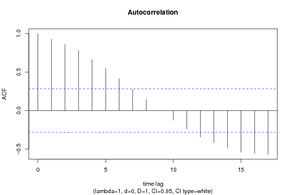
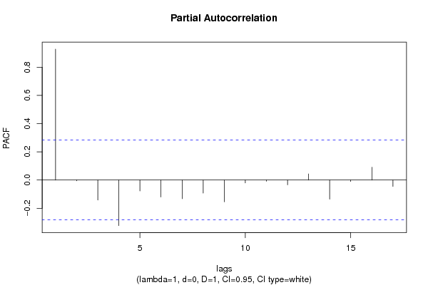
Title produced by software

(Partial) Autocorrelation Function

Date of computation

Thu, 06 Jan 2011 12:52:41 +0000

Cite this page as follows

Statistical Computations at FreeStatistics.org, Office for Research Development and Education, URL https://freestatistics.org/blog/index.php?v=date/2011/Jan/06/t129431822765fiaouxvud2du8.htm/, Retrieved Thu, 16 May 2024 23:44:10 +0000

Statistical Computations at FreeStatistics.org, Office for Research Development and Education, URL https://freestatistics.org/blog/index.php?pk=117285, Retrieved Thu, 16 May 2024 23:44:10 +0000

QR Codes:

Paste this QR Code to cite your computation.

Original text written by user:

IsPrivate?

No (this computation is public)

User-defined keywords

Estimated Impact

264

Family? (F = Feedback message, R = changed R code, M = changed R Module, P = changed Parameters, D = changed Data)

-     [Univariate Data Series] [data set] [2008-12-01 19:54:57] [b98453cac15ba1066b407e146608df68]
- RMP   [(Partial) Autocorrelation Function] [Unemployment] [2010-11-29 09:05:21] [b98453cac15ba1066b407e146608df68]
-    D    [(Partial) Autocorrelation Function] [Workshop 6 'Aanta...] [2010-12-14 16:26:00] [40c8b935cbad1b0be3c22a481f9723f7]
-           [(Partial) Autocorrelation Function] [] [2010-12-16 00:41:10] [bcc4ad4a6c0f95d5b548de29638ac6c2]
-   P         [(Partial) Autocorrelation Function] [] [2010-12-16 01:31:32] [bcc4ad4a6c0f95d5b548de29638ac6c2]
-               [(Partial) Autocorrelation Function] [ACF] [2010-12-16 17:57:21] [f1aa04283d83c25edc8ae3bb0d0fb93e]
-    D            [(Partial) Autocorrelation Function] [autocorrelatie] [2010-12-27 14:52:24] [f1aa04283d83c25edc8ae3bb0d0fb93e]
- R P               [(Partial) Autocorrelation Function] [autocorrelatie] [2010-12-29 20:05:52] [99820e5c3330fe494c612533a1ea567a]
-   P                   [(Partial) Autocorrelation Function] [ACF met alleen D=0] [2011-01-06 12:52:41] [03bcd8c83ef1a42b4029a16ba47a4880] [Current]

Feedback Forum

Post a new message

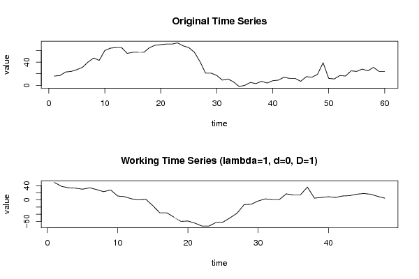
Dataseries X:

Download CSV

Histogram

Boxplots

Summary of computational transaction
Raw Input	view raw input (R code)
Raw Output	view raw output of R engine
Computing time	1 seconds
R Server	'Herman Ole Andreas Wold' @ www.yougetit.org

\begin{tabular}{lllllllll}
\hline
Summary of computational transaction \tabularnewline
Raw Input & view raw input (R code)  \tabularnewline
Raw Output & view raw output of R engine  \tabularnewline
Computing time & 1 seconds \tabularnewline
R Server & 'Herman Ole Andreas Wold' @ www.yougetit.org \tabularnewline
\hline
\end{tabular}
%Source: https://freestatistics.org/blog/index.php?pk=117285&T=0

[TABLE]
[ROW][C]Summary of computational transaction[/C][/ROW]
[ROW][C]Raw Input[/C][C]view raw input (R code) [/C][/ROW]
[ROW][C]Raw Output[/C][C]view raw output of R engine [/C][/ROW]
[ROW][C]Computing time[/C][C]1 seconds[/C][/ROW]
[ROW][C]R Server[/C][C]'Herman Ole Andreas Wold' @ www.yougetit.org[/C][/ROW]
[/TABLE]
Source: https://freestatistics.org/blog/index.php?pk=117285&T=0

Globally Unique Identifier (entire table): ba.freestatistics.org/blog/index.php?pk=117285&T=0

As an alternative you can also use a QR Code:

The GUIDs for individual cells are displayed in the table below:

Summary of computational transaction
Raw Input	view raw input (R code)
Raw Output	view raw output of R engine
Computing time	1 seconds
R Server	'Herman Ole Andreas Wold' @ www.yougetit.org

Autocorrelation Function
Time lag k	ACF(k)	T-STAT	P-value
1	0.928379	6.432	0
2	0.861104	5.9659	0
3	0.779077	5.3976	1e-06
4	0.660489	4.576	1.7e-05
5	0.54459	3.773	0.000222
6	0.417311	2.8912	0.002875
7	0.278797	1.9316	0.029665
8	0.144573	1.0016	0.160772
9	0.002552	0.0177	0.492984
10	-0.125347	-0.8684	0.194741
11	-0.238216	-1.6504	0.052694
12	-0.341925	-2.3689	0.010956
13	-0.417177	-2.8903	0.002882
14	-0.490473	-3.3981	0.000686
15	-0.541055	-3.7485	0.000239
16	-0.556908	-3.8584	0.00017
17	-0.568484	-3.9386	0.000132

\begin{tabular}{lllllllll}
\hline
Autocorrelation Function \tabularnewline
Time lag k & ACF(k) & T-STAT & P-value \tabularnewline
1 & 0.928379 & 6.432 & 0 \tabularnewline
2 & 0.861104 & 5.9659 & 0 \tabularnewline
3 & 0.779077 & 5.3976 & 1e-06 \tabularnewline
4 & 0.660489 & 4.576 & 1.7e-05 \tabularnewline
5 & 0.54459 & 3.773 & 0.000222 \tabularnewline
6 & 0.417311 & 2.8912 & 0.002875 \tabularnewline
7 & 0.278797 & 1.9316 & 0.029665 \tabularnewline
8 & 0.144573 & 1.0016 & 0.160772 \tabularnewline
9 & 0.002552 & 0.0177 & 0.492984 \tabularnewline
10 & -0.125347 & -0.8684 & 0.194741 \tabularnewline
11 & -0.238216 & -1.6504 & 0.052694 \tabularnewline
12 & -0.341925 & -2.3689 & 0.010956 \tabularnewline
13 & -0.417177 & -2.8903 & 0.002882 \tabularnewline
14 & -0.490473 & -3.3981 & 0.000686 \tabularnewline
15 & -0.541055 & -3.7485 & 0.000239 \tabularnewline
16 & -0.556908 & -3.8584 & 0.00017 \tabularnewline
17 & -0.568484 & -3.9386 & 0.000132 \tabularnewline
\hline
\end{tabular}
%Source: https://freestatistics.org/blog/index.php?pk=117285&T=1

[TABLE]
[ROW][C]Autocorrelation Function[/C][/ROW]
[ROW][C]Time lag k[/C][C]ACF(k)[/C][C]T-STAT[/C][C]P-value[/C][/ROW]
[ROW][C]1[/C][C]0.928379[/C][C]6.432[/C][C]0[/C][/ROW]
[ROW][C]2[/C][C]0.861104[/C][C]5.9659[/C][C]0[/C][/ROW]
[ROW][C]3[/C][C]0.779077[/C][C]5.3976[/C][C]1e-06[/C][/ROW]
[ROW][C]4[/C][C]0.660489[/C][C]4.576[/C][C]1.7e-05[/C][/ROW]
[ROW][C]5[/C][C]0.54459[/C][C]3.773[/C][C]0.000222[/C][/ROW]
[ROW][C]6[/C][C]0.417311[/C][C]2.8912[/C][C]0.002875[/C][/ROW]
[ROW][C]7[/C][C]0.278797[/C][C]1.9316[/C][C]0.029665[/C][/ROW]
[ROW][C]8[/C][C]0.144573[/C][C]1.0016[/C][C]0.160772[/C][/ROW]
[ROW][C]9[/C][C]0.002552[/C][C]0.0177[/C][C]0.492984[/C][/ROW]
[ROW][C]10[/C][C]-0.125347[/C][C]-0.8684[/C][C]0.194741[/C][/ROW]
[ROW][C]11[/C][C]-0.238216[/C][C]-1.6504[/C][C]0.052694[/C][/ROW]
[ROW][C]12[/C][C]-0.341925[/C][C]-2.3689[/C][C]0.010956[/C][/ROW]
[ROW][C]13[/C][C]-0.417177[/C][C]-2.8903[/C][C]0.002882[/C][/ROW]
[ROW][C]14[/C][C]-0.490473[/C][C]-3.3981[/C][C]0.000686[/C][/ROW]
[ROW][C]15[/C][C]-0.541055[/C][C]-3.7485[/C][C]0.000239[/C][/ROW]
[ROW][C]16[/C][C]-0.556908[/C][C]-3.8584[/C][C]0.00017[/C][/ROW]
[ROW][C]17[/C][C]-0.568484[/C][C]-3.9386[/C][C]0.000132[/C][/ROW]
[/TABLE]
Source: https://freestatistics.org/blog/index.php?pk=117285&T=1

Globally Unique Identifier (entire table): ba.freestatistics.org/blog/index.php?pk=117285&T=1

As an alternative you can also use a QR Code:

The GUIDs for individual cells are displayed in the table below:

Autocorrelation Function
Time lag k	ACF(k)	T-STAT	P-value
1	0.928379	6.432	0
2	0.861104	5.9659	0
3	0.779077	5.3976	1e-06
4	0.660489	4.576	1.7e-05
5	0.54459	3.773	0.000222
6	0.417311	2.8912	0.002875
7	0.278797	1.9316	0.029665
8	0.144573	1.0016	0.160772
9	0.002552	0.0177	0.492984
10	-0.125347	-0.8684	0.194741
11	-0.238216	-1.6504	0.052694
12	-0.341925	-2.3689	0.010956
13	-0.417177	-2.8903	0.002882
14	-0.490473	-3.3981	0.000686
15	-0.541055	-3.7485	0.000239
16	-0.556908	-3.8584	0.00017
17	-0.568484	-3.9386	0.000132

Partial Autocorrelation Function
Time lag k	PACF(k)	T-STAT	P-value
1	0.928379	6.432	0
2	-0.005671	-0.0393	0.484412
3	-0.142075	-0.9843	0.164946
4	-0.322968	-2.2376	0.014962
5	-0.077211	-0.5349	0.297582
6	-0.120528	-0.835	0.203915
7	-0.132176	-0.9157	0.18219
8	-0.09252	-0.641	0.262287
9	-0.153851	-1.0659	0.145898
10	-0.020509	-0.1421	0.4438
11	-0.008536	-0.0591	0.476543
12	-0.033785	-0.2341	0.407962
13	0.043671	0.3026	0.381764
14	-0.135746	-0.9405	0.175842
15	-0.01003	-0.0695	0.472444
16	0.090646	0.628	0.266486
17	-0.045054	-0.3121	0.378141

\begin{tabular}{lllllllll}
\hline
Partial Autocorrelation Function \tabularnewline
Time lag k & PACF(k) & T-STAT & P-value \tabularnewline
1 & 0.928379 & 6.432 & 0 \tabularnewline
2 & -0.005671 & -0.0393 & 0.484412 \tabularnewline
3 & -0.142075 & -0.9843 & 0.164946 \tabularnewline
4 & -0.322968 & -2.2376 & 0.014962 \tabularnewline
5 & -0.077211 & -0.5349 & 0.297582 \tabularnewline
6 & -0.120528 & -0.835 & 0.203915 \tabularnewline
7 & -0.132176 & -0.9157 & 0.18219 \tabularnewline
8 & -0.09252 & -0.641 & 0.262287 \tabularnewline
9 & -0.153851 & -1.0659 & 0.145898 \tabularnewline
10 & -0.020509 & -0.1421 & 0.4438 \tabularnewline
11 & -0.008536 & -0.0591 & 0.476543 \tabularnewline
12 & -0.033785 & -0.2341 & 0.407962 \tabularnewline
13 & 0.043671 & 0.3026 & 0.381764 \tabularnewline
14 & -0.135746 & -0.9405 & 0.175842 \tabularnewline
15 & -0.01003 & -0.0695 & 0.472444 \tabularnewline
16 & 0.090646 & 0.628 & 0.266486 \tabularnewline
17 & -0.045054 & -0.3121 & 0.378141 \tabularnewline
\hline
\end{tabular}
%Source: https://freestatistics.org/blog/index.php?pk=117285&T=2

[TABLE]
[ROW][C]Partial Autocorrelation Function[/C][/ROW]
[ROW][C]Time lag k[/C][C]PACF(k)[/C][C]T-STAT[/C][C]P-value[/C][/ROW]
[ROW][C]1[/C][C]0.928379[/C][C]6.432[/C][C]0[/C][/ROW]
[ROW][C]2[/C][C]-0.005671[/C][C]-0.0393[/C][C]0.484412[/C][/ROW]
[ROW][C]3[/C][C]-0.142075[/C][C]-0.9843[/C][C]0.164946[/C][/ROW]
[ROW][C]4[/C][C]-0.322968[/C][C]-2.2376[/C][C]0.014962[/C][/ROW]
[ROW][C]5[/C][C]-0.077211[/C][C]-0.5349[/C][C]0.297582[/C][/ROW]
[ROW][C]6[/C][C]-0.120528[/C][C]-0.835[/C][C]0.203915[/C][/ROW]
[ROW][C]7[/C][C]-0.132176[/C][C]-0.9157[/C][C]0.18219[/C][/ROW]
[ROW][C]8[/C][C]-0.09252[/C][C]-0.641[/C][C]0.262287[/C][/ROW]
[ROW][C]9[/C][C]-0.153851[/C][C]-1.0659[/C][C]0.145898[/C][/ROW]
[ROW][C]10[/C][C]-0.020509[/C][C]-0.1421[/C][C]0.4438[/C][/ROW]
[ROW][C]11[/C][C]-0.008536[/C][C]-0.0591[/C][C]0.476543[/C][/ROW]
[ROW][C]12[/C][C]-0.033785[/C][C]-0.2341[/C][C]0.407962[/C][/ROW]
[ROW][C]13[/C][C]0.043671[/C][C]0.3026[/C][C]0.381764[/C][/ROW]
[ROW][C]14[/C][C]-0.135746[/C][C]-0.9405[/C][C]0.175842[/C][/ROW]
[ROW][C]15[/C][C]-0.01003[/C][C]-0.0695[/C][C]0.472444[/C][/ROW]
[ROW][C]16[/C][C]0.090646[/C][C]0.628[/C][C]0.266486[/C][/ROW]
[ROW][C]17[/C][C]-0.045054[/C][C]-0.3121[/C][C]0.378141[/C][/ROW]
[/TABLE]
Source: https://freestatistics.org/blog/index.php?pk=117285&T=2

Globally Unique Identifier (entire table): ba.freestatistics.org/blog/index.php?pk=117285&T=2

As an alternative you can also use a QR Code:

The GUIDs for individual cells are displayed in the table below:

Partial Autocorrelation Function
Time lag k	PACF(k)	T-STAT	P-value
1	0.928379	6.432	0
2	-0.005671	-0.0393	0.484412
3	-0.142075	-0.9843	0.164946
4	-0.322968	-2.2376	0.014962
5	-0.077211	-0.5349	0.297582
6	-0.120528	-0.835	0.203915
7	-0.132176	-0.9157	0.18219
8	-0.09252	-0.641	0.262287
9	-0.153851	-1.0659	0.145898
10	-0.020509	-0.1421	0.4438
11	-0.008536	-0.0591	0.476543
12	-0.033785	-0.2341	0.407962
13	0.043671	0.3026	0.381764
14	-0.135746	-0.9405	0.175842
15	-0.01003	-0.0695	0.472444
16	0.090646	0.628	0.266486
17	-0.045054	-0.3121	0.378141

Figure 1

PNG link

Postscript link

PDF link

Figure 2

PNG link

Postscript link

PDF link

Figure 3

PNG link

Postscript link

PDF link

Parameters (Session):

par1 = Default ; par2 = 1 ; par3 = 0 ; par4 = 1 ; par5 = 12 ; par6 = White Noise ; par7 = 0.95 ;

Parameters (R input):

par1 = Default ; par2 = 1 ; par3 = 0 ; par4 = 1 ; par5 = 12 ; par6 = White Noise ; par7 = 0.95 ; par8 = ;

R code (references can be found in the software module):

if (par1 == 'Default') {
par1 = 10*log10(length(x))
} else {
par1 <- as.numeric(par1)
}
par2 <- as.numeric(par2)
par3 <- as.numeric(par3)
par4 <- as.numeric(par4)
par5 <- as.numeric(par5)
if (par6 == 'White Noise') par6 <- 'white' else par6 <- 'ma'
par7 <- as.numeric(par7)
if (par8 != '') par8 <- as.numeric(par8)
ox <- x
if (par8 == '') {
if (par2 == 0) {
x <- log(x)
} else {
x <- (x ^ par2 - 1) / par2
}
} else {
x <- log(x,base=par8)
}
if (par3 > 0) x <- diff(x,lag=1,difference=par3)
if (par4 > 0) x <- diff(x,lag=par5,difference=par4)
bitmap(file='picts.png')
op <- par(mfrow=c(2,1))
plot(ox,type='l',main='Original Time Series',xlab='time',ylab='value')
if (par8=='') {
mytitle <- paste('Working Time Series (lambda=',par2,', d=',par3,', D=',par4,')',sep='')
mysub <- paste('(lambda=',par2,', d=',par3,', D=',par4,', CI=', par7, ', CI type=',par6,')',sep='')
} else {
mytitle <- paste('Working Time Series (base=',par8,', d=',par3,', D=',par4,')',sep='')
mysub <- paste('(base=',par8,', d=',par3,', D=',par4,', CI=', par7, ', CI type=',par6,')',sep='')
}
plot(x,type='l', main=mytitle,xlab='time',ylab='value')
par(op)
dev.off()
bitmap(file='pic1.png')
racf <- acf(x, par1, main='Autocorrelation', xlab='time lag', ylab='ACF', ci.type=par6, ci=par7, sub=mysub)
dev.off()
bitmap(file='pic2.png')
rpacf <- pacf(x,par1,main='Partial Autocorrelation',xlab='lags',ylab='PACF',sub=mysub)
dev.off()
(myacf <- c(racf$acf))
(mypacf <- c(rpacf$acf))
lengthx <- length(x)
sqrtn <- sqrt(lengthx)
load(file='createtable')
a<-table.start()
a<-table.row.start(a)
a<-table.element(a,'Autocorrelation Function',4,TRUE)
a<-table.row.end(a)
a<-table.row.start(a)
a<-table.element(a,'Time lag k',header=TRUE)
a<-table.element(a,hyperlink('basics.htm','ACF(k)','click here for more information about the Autocorrelation Function'),header=TRUE)
a<-table.element(a,'T-STAT',header=TRUE)
a<-table.element(a,'P-value',header=TRUE)
a<-table.row.end(a)
for (i in 2:(par1+1)) {
a<-table.row.start(a)
a<-table.element(a,i-1,header=TRUE)
a<-table.element(a,round(myacf[i],6))
mytstat <- myacf[i]*sqrtn
a<-table.element(a,round(mytstat,4))
a<-table.element(a,round(1-pt(abs(mytstat),lengthx),6))
a<-table.row.end(a)
}
a<-table.end(a)
table.save(a,file='mytable.tab')
a<-table.start()
a<-table.row.start(a)
a<-table.element(a,'Partial Autocorrelation Function',4,TRUE)
a<-table.row.end(a)
a<-table.row.start(a)
a<-table.element(a,'Time lag k',header=TRUE)
a<-table.element(a,hyperlink('basics.htm','PACF(k)','click here for more information about the Partial Autocorrelation Function'),header=TRUE)
a<-table.element(a,'T-STAT',header=TRUE)
a<-table.element(a,'P-value',header=TRUE)
a<-table.row.end(a)
for (i in 1:par1) {
a<-table.row.start(a)
a<-table.element(a,i,header=TRUE)
a<-table.element(a,round(mypacf[i],6))
mytstat <- mypacf[i]*sqrtn
a<-table.element(a,round(mytstat,4))
a<-table.element(a,round(1-pt(abs(mytstat),lengthx),6))
a<-table.row.end(a)
}
a<-table.end(a)
table.save(a,file='mytable1.tab')

Free Statistics

Description of Statistical Computation

Tree of Dependent Computations

Dataset

Tables (Output of Computation)

Figures (Output of Computation)

Input Parameters & R Code