Repository of Reproducible Computations

Free Statistics

of Irreproducible Research!

Author's title

Author

*Unverified author*

R Software Module

rwasp_exponentialsmoothing.wasp

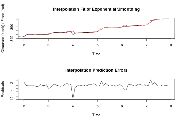
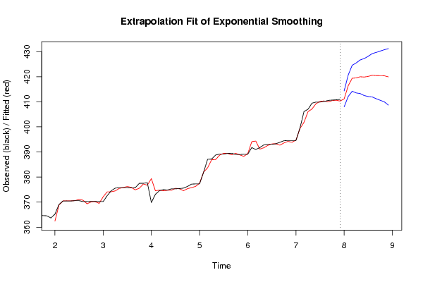
Title produced by software

Exponential Smoothing

Date of computation

Thu, 06 Jan 2011 18:55:40 +0000

Cite this page as follows

Statistical Computations at FreeStatistics.org, Office for Research Development and Education, URL https://freestatistics.org/blog/index.php?v=date/2011/Jan/06/t1294340015ff8spkuokt453wa.htm/, Retrieved Thu, 16 May 2024 18:54:57 +0000

Statistical Computations at FreeStatistics.org, Office for Research Development and Education, URL https://freestatistics.org/blog/index.php?pk=117290, Retrieved Thu, 16 May 2024 18:54:57 +0000

QR Codes:

Paste this QR Code to cite your computation.

Original text written by user:

Eigen tijdreeks

IsPrivate?

No (this computation is public)

User-defined keywords

KDGP2W102

Estimated Impact

205

Family? (F = Feedback message, R = changed R code, M = changed R Module, P = changed Parameters, D = changed Data)

-       [Exponential Smoothing] [Opdracht 10] [2011-01-06 18:55:40] [cf38f7df7be58a8c28b053c2e6c1601e] [Current]

Feedback Forum

Post a new message

Dataseries X:

Download CSV

Histogram

Boxplots

Summary of computational transaction
Raw Input	view raw input (R code)
Raw Output	view raw output of R engine
Computing time	2 seconds
R Server	'Sir Ronald Aylmer Fisher' @ 193.190.124.24

\begin{tabular}{lllllllll}
\hline
Summary of computational transaction \tabularnewline
Raw Input & view raw input (R code)  \tabularnewline
Raw Output & view raw output of R engine  \tabularnewline
Computing time & 2 seconds \tabularnewline
R Server & 'Sir Ronald Aylmer Fisher' @ 193.190.124.24 \tabularnewline
\hline
\end{tabular}
%Source: https://freestatistics.org/blog/index.php?pk=117290&T=0

[TABLE]
[ROW][C]Summary of computational transaction[/C][/ROW]
[ROW][C]Raw Input[/C][C]view raw input (R code) [/C][/ROW]
[ROW][C]Raw Output[/C][C]view raw output of R engine [/C][/ROW]
[ROW][C]Computing time[/C][C]2 seconds[/C][/ROW]
[ROW][C]R Server[/C][C]'Sir Ronald Aylmer Fisher' @ 193.190.124.24[/C][/ROW]
[/TABLE]
Source: https://freestatistics.org/blog/index.php?pk=117290&T=0

Globally Unique Identifier (entire table): ba.freestatistics.org/blog/index.php?pk=117290&T=0

As an alternative you can also use a QR Code:

The GUIDs for individual cells are displayed in the table below:

Summary of computational transaction
Raw Input	view raw input (R code)
Raw Output	view raw output of R engine
Computing time	2 seconds
R Server	'Sir Ronald Aylmer Fisher' @ 193.190.124.24

Estimated Parameters of Exponential Smoothing
Parameter	Value
alpha	0.883046242290146
beta	0.0232953695718167
gamma	1

\begin{tabular}{lllllllll}
\hline
Estimated Parameters of Exponential Smoothing \tabularnewline
Parameter & Value \tabularnewline
alpha & 0.883046242290146 \tabularnewline
beta & 0.0232953695718167 \tabularnewline
gamma & 1 \tabularnewline
\hline
\end{tabular}
%Source: https://freestatistics.org/blog/index.php?pk=117290&T=1

[TABLE]
[ROW][C]Estimated Parameters of Exponential Smoothing[/C][/ROW]
[ROW][C]Parameter[/C][C]Value[/C][/ROW]
[ROW][C]alpha[/C][C]0.883046242290146[/C][/ROW]
[ROW][C]beta[/C][C]0.0232953695718167[/C][/ROW]
[ROW][C]gamma[/C][C]1[/C][/ROW]
[/TABLE]
Source: https://freestatistics.org/blog/index.php?pk=117290&T=1

Globally Unique Identifier (entire table): ba.freestatistics.org/blog/index.php?pk=117290&T=1

As an alternative you can also use a QR Code:

The GUIDs for individual cells are displayed in the table below:

Estimated Parameters of Exponential Smoothing
Parameter	Value
alpha	0.883046242290146
beta	0.0232953695718167
gamma	1

Interpolation Forecasts of Exponential Smoothing
t	Observed	Fitted	Residuals
13	365.22	362.446094114382	2.77390588561815
14	369.05	368.828279220148	0.221720779852205
15	370.45	370.511943494574	-0.0619434945735975
16	370.46	370.514428569369	-0.0544285693695201
17	370.46	370.506934160959	-0.0469341609594949
18	370.58	370.588702684452	-0.00870268445248712
19	370.58	371.110917019533	-0.530917019532637
20	370.22	370.744672684485	-0.524672684484756
21	370.21	369.316498369238	0.893501630762216
22	370.29	370.101096265564	0.188903734436224
23	370.29	370.214827639326	0.0751723606742303
24	370.2	369.489537053875	0.710462946125404
25	370.2	372.125612277186	-1.92561227718613
26	372.55	374.08194541213	-1.53194541212969
27	374.51	374.135041223477	0.374958776523385
28	375.58	374.470127750496	1.10987224950367
29	375.75	375.460129018177	0.289870981822673
30	375.75	375.820122163439	-0.0701221634388389
31	375.75	376.206877243224	-0.45687724322363
32	375.69	375.883141885205	-0.193141885205421
33	375.76	374.88319364792	0.876806352079825
34	377.5	375.550515370813	1.94948462918722
35	377.51	377.219534972011	0.290465027989342
36	377.74	376.763812735547	0.976187264452676
37	369.82	379.383421653442	-9.56342165344176
38	373.1	374.523545441961	-1.42354544196075
39	374.55	374.775959409283	-0.225959409283348
40	375.01	374.532099668686	0.477900331314174
41	374.81	374.72244564073	0.0875543592703139
42	375.31	374.712161794589	0.597838205411279
43	375.31	375.506746545563	-0.196746545562917
44	375.39	375.312605196631	0.0773948033691454
45	375.59	374.552048354121	1.03795164587893
46	376.26	375.364518143143	0.895481856857316
47	377.18	375.768201260077	1.41179873992292
48	377.26	376.264241246982	0.995758753018151
49	377.26	377.523632457265	-0.263632457265430
50	381.87	381.98352585277	-0.113525852770124
51	387.09	383.66288966868	3.42711033132031
52	387.14	386.891742293209	0.248257706790525
53	388.78	386.982839246401	1.7971607535992
54	389.16	388.732280720722	0.427719279278222
55	389.16	389.477534014307	-0.317534014306943
56	389.42	389.394078980854	0.0259210191463239
57	389.49	388.856409616119	0.633590383880971
58	388.97	389.464412763687	-0.49441276368691
59	388.97	388.835011309532	0.134988690467878
60	389.09	388.248701821541	0.841298178458999
61	389.09	389.346813542291	-0.256813542291411
62	391.76	394.095009697957	-2.33500969795716
63	390.96	394.355436559733	-3.3954365597329
64	391.76	391.125280432054	0.634719567945638
65	392.8	391.685407644232	1.11459235576831
66	393.06	392.605343823868	0.45465617613246
67	393.06	393.223969271839	-0.163969271838766
68	393.26	393.255847240767	0.00415275923313629
69	393.87	392.702096060566	1.16790393943450
70	394.47	393.596391925323	0.873608074677406
71	394.57	394.220978079186	0.34902192081438
72	394.57	393.875392033645	0.694607966354738
73	394.57	394.693870848066	-0.123870848065678
74	399.57	399.359405963993	0.210594036006796
75	406.13	401.812027963801	4.31797203619863
76	407.03	406.052967098998	0.977032901001735
77	409.46	407.158698189535	2.30130181046508
78	409.9	409.250482824444	0.649517175555502
79	409.9	410.185034367644	-0.285034367644471
80	410.14	410.345491252696	-0.205491252696163
81	410.54	409.926813607666	0.613186392334114
82	410.69	410.479644526196	0.210355473804498
83	410.79	410.624686274348	0.165313725651799
84	410.97	410.303471573743	0.666528426256889

\begin{tabular}{lllllllll}
\hline
Interpolation Forecasts of Exponential Smoothing \tabularnewline
t & Observed & Fitted & Residuals \tabularnewline
13 & 365.22 & 362.446094114382 & 2.77390588561815 \tabularnewline
14 & 369.05 & 368.828279220148 & 0.221720779852205 \tabularnewline
15 & 370.45 & 370.511943494574 & -0.0619434945735975 \tabularnewline
16 & 370.46 & 370.514428569369 & -0.0544285693695201 \tabularnewline
17 & 370.46 & 370.506934160959 & -0.0469341609594949 \tabularnewline
18 & 370.58 & 370.588702684452 & -0.00870268445248712 \tabularnewline
19 & 370.58 & 371.110917019533 & -0.530917019532637 \tabularnewline
20 & 370.22 & 370.744672684485 & -0.524672684484756 \tabularnewline
21 & 370.21 & 369.316498369238 & 0.893501630762216 \tabularnewline
22 & 370.29 & 370.101096265564 & 0.188903734436224 \tabularnewline
23 & 370.29 & 370.214827639326 & 0.0751723606742303 \tabularnewline
24 & 370.2 & 369.489537053875 & 0.710462946125404 \tabularnewline
25 & 370.2 & 372.125612277186 & -1.92561227718613 \tabularnewline
26 & 372.55 & 374.08194541213 & -1.53194541212969 \tabularnewline
27 & 374.51 & 374.135041223477 & 0.374958776523385 \tabularnewline
28 & 375.58 & 374.470127750496 & 1.10987224950367 \tabularnewline
29 & 375.75 & 375.460129018177 & 0.289870981822673 \tabularnewline
30 & 375.75 & 375.820122163439 & -0.0701221634388389 \tabularnewline
31 & 375.75 & 376.206877243224 & -0.45687724322363 \tabularnewline
32 & 375.69 & 375.883141885205 & -0.193141885205421 \tabularnewline
33 & 375.76 & 374.88319364792 & 0.876806352079825 \tabularnewline
34 & 377.5 & 375.550515370813 & 1.94948462918722 \tabularnewline
35 & 377.51 & 377.219534972011 & 0.290465027989342 \tabularnewline
36 & 377.74 & 376.763812735547 & 0.976187264452676 \tabularnewline
37 & 369.82 & 379.383421653442 & -9.56342165344176 \tabularnewline
38 & 373.1 & 374.523545441961 & -1.42354544196075 \tabularnewline
39 & 374.55 & 374.775959409283 & -0.225959409283348 \tabularnewline
40 & 375.01 & 374.532099668686 & 0.477900331314174 \tabularnewline
41 & 374.81 & 374.72244564073 & 0.0875543592703139 \tabularnewline
42 & 375.31 & 374.712161794589 & 0.597838205411279 \tabularnewline
43 & 375.31 & 375.506746545563 & -0.196746545562917 \tabularnewline
44 & 375.39 & 375.312605196631 & 0.0773948033691454 \tabularnewline
45 & 375.59 & 374.552048354121 & 1.03795164587893 \tabularnewline
46 & 376.26 & 375.364518143143 & 0.895481856857316 \tabularnewline
47 & 377.18 & 375.768201260077 & 1.41179873992292 \tabularnewline
48 & 377.26 & 376.264241246982 & 0.995758753018151 \tabularnewline
49 & 377.26 & 377.523632457265 & -0.263632457265430 \tabularnewline
50 & 381.87 & 381.98352585277 & -0.113525852770124 \tabularnewline
51 & 387.09 & 383.66288966868 & 3.42711033132031 \tabularnewline
52 & 387.14 & 386.891742293209 & 0.248257706790525 \tabularnewline
53 & 388.78 & 386.982839246401 & 1.7971607535992 \tabularnewline
54 & 389.16 & 388.732280720722 & 0.427719279278222 \tabularnewline
55 & 389.16 & 389.477534014307 & -0.317534014306943 \tabularnewline
56 & 389.42 & 389.394078980854 & 0.0259210191463239 \tabularnewline
57 & 389.49 & 388.856409616119 & 0.633590383880971 \tabularnewline
58 & 388.97 & 389.464412763687 & -0.49441276368691 \tabularnewline
59 & 388.97 & 388.835011309532 & 0.134988690467878 \tabularnewline
60 & 389.09 & 388.248701821541 & 0.841298178458999 \tabularnewline
61 & 389.09 & 389.346813542291 & -0.256813542291411 \tabularnewline
62 & 391.76 & 394.095009697957 & -2.33500969795716 \tabularnewline
63 & 390.96 & 394.355436559733 & -3.3954365597329 \tabularnewline
64 & 391.76 & 391.125280432054 & 0.634719567945638 \tabularnewline
65 & 392.8 & 391.685407644232 & 1.11459235576831 \tabularnewline
66 & 393.06 & 392.605343823868 & 0.45465617613246 \tabularnewline
67 & 393.06 & 393.223969271839 & -0.163969271838766 \tabularnewline
68 & 393.26 & 393.255847240767 & 0.00415275923313629 \tabularnewline
69 & 393.87 & 392.702096060566 & 1.16790393943450 \tabularnewline
70 & 394.47 & 393.596391925323 & 0.873608074677406 \tabularnewline
71 & 394.57 & 394.220978079186 & 0.34902192081438 \tabularnewline
72 & 394.57 & 393.875392033645 & 0.694607966354738 \tabularnewline
73 & 394.57 & 394.693870848066 & -0.123870848065678 \tabularnewline
74 & 399.57 & 399.359405963993 & 0.210594036006796 \tabularnewline
75 & 406.13 & 401.812027963801 & 4.31797203619863 \tabularnewline
76 & 407.03 & 406.052967098998 & 0.977032901001735 \tabularnewline
77 & 409.46 & 407.158698189535 & 2.30130181046508 \tabularnewline
78 & 409.9 & 409.250482824444 & 0.649517175555502 \tabularnewline
79 & 409.9 & 410.185034367644 & -0.285034367644471 \tabularnewline
80 & 410.14 & 410.345491252696 & -0.205491252696163 \tabularnewline
81 & 410.54 & 409.926813607666 & 0.613186392334114 \tabularnewline
82 & 410.69 & 410.479644526196 & 0.210355473804498 \tabularnewline
83 & 410.79 & 410.624686274348 & 0.165313725651799 \tabularnewline
84 & 410.97 & 410.303471573743 & 0.666528426256889 \tabularnewline
\hline
\end{tabular}
%Source: https://freestatistics.org/blog/index.php?pk=117290&T=2

[TABLE]
[ROW][C]Interpolation Forecasts of Exponential Smoothing[/C][/ROW]
[ROW][C]t[/C][C]Observed[/C][C]Fitted[/C][C]Residuals[/C][/ROW]
[ROW][C]13[/C][C]365.22[/C][C]362.446094114382[/C][C]2.77390588561815[/C][/ROW]
[ROW][C]14[/C][C]369.05[/C][C]368.828279220148[/C][C]0.221720779852205[/C][/ROW]
[ROW][C]15[/C][C]370.45[/C][C]370.511943494574[/C][C]-0.0619434945735975[/C][/ROW]
[ROW][C]16[/C][C]370.46[/C][C]370.514428569369[/C][C]-0.0544285693695201[/C][/ROW]
[ROW][C]17[/C][C]370.46[/C][C]370.506934160959[/C][C]-0.0469341609594949[/C][/ROW]
[ROW][C]18[/C][C]370.58[/C][C]370.588702684452[/C][C]-0.00870268445248712[/C][/ROW]
[ROW][C]19[/C][C]370.58[/C][C]371.110917019533[/C][C]-0.530917019532637[/C][/ROW]
[ROW][C]20[/C][C]370.22[/C][C]370.744672684485[/C][C]-0.524672684484756[/C][/ROW]
[ROW][C]21[/C][C]370.21[/C][C]369.316498369238[/C][C]0.893501630762216[/C][/ROW]
[ROW][C]22[/C][C]370.29[/C][C]370.101096265564[/C][C]0.188903734436224[/C][/ROW]
[ROW][C]23[/C][C]370.29[/C][C]370.214827639326[/C][C]0.0751723606742303[/C][/ROW]
[ROW][C]24[/C][C]370.2[/C][C]369.489537053875[/C][C]0.710462946125404[/C][/ROW]
[ROW][C]25[/C][C]370.2[/C][C]372.125612277186[/C][C]-1.92561227718613[/C][/ROW]
[ROW][C]26[/C][C]372.55[/C][C]374.08194541213[/C][C]-1.53194541212969[/C][/ROW]
[ROW][C]27[/C][C]374.51[/C][C]374.135041223477[/C][C]0.374958776523385[/C][/ROW]
[ROW][C]28[/C][C]375.58[/C][C]374.470127750496[/C][C]1.10987224950367[/C][/ROW]
[ROW][C]29[/C][C]375.75[/C][C]375.460129018177[/C][C]0.289870981822673[/C][/ROW]
[ROW][C]30[/C][C]375.75[/C][C]375.820122163439[/C][C]-0.0701221634388389[/C][/ROW]
[ROW][C]31[/C][C]375.75[/C][C]376.206877243224[/C][C]-0.45687724322363[/C][/ROW]
[ROW][C]32[/C][C]375.69[/C][C]375.883141885205[/C][C]-0.193141885205421[/C][/ROW]
[ROW][C]33[/C][C]375.76[/C][C]374.88319364792[/C][C]0.876806352079825[/C][/ROW]
[ROW][C]34[/C][C]377.5[/C][C]375.550515370813[/C][C]1.94948462918722[/C][/ROW]
[ROW][C]35[/C][C]377.51[/C][C]377.219534972011[/C][C]0.290465027989342[/C][/ROW]
[ROW][C]36[/C][C]377.74[/C][C]376.763812735547[/C][C]0.976187264452676[/C][/ROW]
[ROW][C]37[/C][C]369.82[/C][C]379.383421653442[/C][C]-9.56342165344176[/C][/ROW]
[ROW][C]38[/C][C]373.1[/C][C]374.523545441961[/C][C]-1.42354544196075[/C][/ROW]
[ROW][C]39[/C][C]374.55[/C][C]374.775959409283[/C][C]-0.225959409283348[/C][/ROW]
[ROW][C]40[/C][C]375.01[/C][C]374.532099668686[/C][C]0.477900331314174[/C][/ROW]
[ROW][C]41[/C][C]374.81[/C][C]374.72244564073[/C][C]0.0875543592703139[/C][/ROW]
[ROW][C]42[/C][C]375.31[/C][C]374.712161794589[/C][C]0.597838205411279[/C][/ROW]
[ROW][C]43[/C][C]375.31[/C][C]375.506746545563[/C][C]-0.196746545562917[/C][/ROW]
[ROW][C]44[/C][C]375.39[/C][C]375.312605196631[/C][C]0.0773948033691454[/C][/ROW]
[ROW][C]45[/C][C]375.59[/C][C]374.552048354121[/C][C]1.03795164587893[/C][/ROW]
[ROW][C]46[/C][C]376.26[/C][C]375.364518143143[/C][C]0.895481856857316[/C][/ROW]
[ROW][C]47[/C][C]377.18[/C][C]375.768201260077[/C][C]1.41179873992292[/C][/ROW]
[ROW][C]48[/C][C]377.26[/C][C]376.264241246982[/C][C]0.995758753018151[/C][/ROW]
[ROW][C]49[/C][C]377.26[/C][C]377.523632457265[/C][C]-0.263632457265430[/C][/ROW]
[ROW][C]50[/C][C]381.87[/C][C]381.98352585277[/C][C]-0.113525852770124[/C][/ROW]
[ROW][C]51[/C][C]387.09[/C][C]383.66288966868[/C][C]3.42711033132031[/C][/ROW]
[ROW][C]52[/C][C]387.14[/C][C]386.891742293209[/C][C]0.248257706790525[/C][/ROW]
[ROW][C]53[/C][C]388.78[/C][C]386.982839246401[/C][C]1.7971607535992[/C][/ROW]
[ROW][C]54[/C][C]389.16[/C][C]388.732280720722[/C][C]0.427719279278222[/C][/ROW]
[ROW][C]55[/C][C]389.16[/C][C]389.477534014307[/C][C]-0.317534014306943[/C][/ROW]
[ROW][C]56[/C][C]389.42[/C][C]389.394078980854[/C][C]0.0259210191463239[/C][/ROW]
[ROW][C]57[/C][C]389.49[/C][C]388.856409616119[/C][C]0.633590383880971[/C][/ROW]
[ROW][C]58[/C][C]388.97[/C][C]389.464412763687[/C][C]-0.49441276368691[/C][/ROW]
[ROW][C]59[/C][C]388.97[/C][C]388.835011309532[/C][C]0.134988690467878[/C][/ROW]
[ROW][C]60[/C][C]389.09[/C][C]388.248701821541[/C][C]0.841298178458999[/C][/ROW]
[ROW][C]61[/C][C]389.09[/C][C]389.346813542291[/C][C]-0.256813542291411[/C][/ROW]
[ROW][C]62[/C][C]391.76[/C][C]394.095009697957[/C][C]-2.33500969795716[/C][/ROW]
[ROW][C]63[/C][C]390.96[/C][C]394.355436559733[/C][C]-3.3954365597329[/C][/ROW]
[ROW][C]64[/C][C]391.76[/C][C]391.125280432054[/C][C]0.634719567945638[/C][/ROW]
[ROW][C]65[/C][C]392.8[/C][C]391.685407644232[/C][C]1.11459235576831[/C][/ROW]
[ROW][C]66[/C][C]393.06[/C][C]392.605343823868[/C][C]0.45465617613246[/C][/ROW]
[ROW][C]67[/C][C]393.06[/C][C]393.223969271839[/C][C]-0.163969271838766[/C][/ROW]
[ROW][C]68[/C][C]393.26[/C][C]393.255847240767[/C][C]0.00415275923313629[/C][/ROW]
[ROW][C]69[/C][C]393.87[/C][C]392.702096060566[/C][C]1.16790393943450[/C][/ROW]
[ROW][C]70[/C][C]394.47[/C][C]393.596391925323[/C][C]0.873608074677406[/C][/ROW]
[ROW][C]71[/C][C]394.57[/C][C]394.220978079186[/C][C]0.34902192081438[/C][/ROW]
[ROW][C]72[/C][C]394.57[/C][C]393.875392033645[/C][C]0.694607966354738[/C][/ROW]
[ROW][C]73[/C][C]394.57[/C][C]394.693870848066[/C][C]-0.123870848065678[/C][/ROW]
[ROW][C]74[/C][C]399.57[/C][C]399.359405963993[/C][C]0.210594036006796[/C][/ROW]
[ROW][C]75[/C][C]406.13[/C][C]401.812027963801[/C][C]4.31797203619863[/C][/ROW]
[ROW][C]76[/C][C]407.03[/C][C]406.052967098998[/C][C]0.977032901001735[/C][/ROW]
[ROW][C]77[/C][C]409.46[/C][C]407.158698189535[/C][C]2.30130181046508[/C][/ROW]
[ROW][C]78[/C][C]409.9[/C][C]409.250482824444[/C][C]0.649517175555502[/C][/ROW]
[ROW][C]79[/C][C]409.9[/C][C]410.185034367644[/C][C]-0.285034367644471[/C][/ROW]
[ROW][C]80[/C][C]410.14[/C][C]410.345491252696[/C][C]-0.205491252696163[/C][/ROW]
[ROW][C]81[/C][C]410.54[/C][C]409.926813607666[/C][C]0.613186392334114[/C][/ROW]
[ROW][C]82[/C][C]410.69[/C][C]410.479644526196[/C][C]0.210355473804498[/C][/ROW]
[ROW][C]83[/C][C]410.79[/C][C]410.624686274348[/C][C]0.165313725651799[/C][/ROW]
[ROW][C]84[/C][C]410.97[/C][C]410.303471573743[/C][C]0.666528426256889[/C][/ROW]
[/TABLE]
Source: https://freestatistics.org/blog/index.php?pk=117290&T=2

Globally Unique Identifier (entire table): ba.freestatistics.org/blog/index.php?pk=117290&T=2

As an alternative you can also use a QR Code:

The GUIDs for individual cells are displayed in the table below:

Interpolation Forecasts of Exponential Smoothing
t	Observed	Fitted	Residuals
13	365.22	362.446094114382	2.77390588561815
14	369.05	368.828279220148	0.221720779852205
15	370.45	370.511943494574	-0.0619434945735975
16	370.46	370.514428569369	-0.0544285693695201
17	370.46	370.506934160959	-0.0469341609594949
18	370.58	370.588702684452	-0.00870268445248712
19	370.58	371.110917019533	-0.530917019532637
20	370.22	370.744672684485	-0.524672684484756
21	370.21	369.316498369238	0.893501630762216
22	370.29	370.101096265564	0.188903734436224
23	370.29	370.214827639326	0.0751723606742303
24	370.2	369.489537053875	0.710462946125404
25	370.2	372.125612277186	-1.92561227718613
26	372.55	374.08194541213	-1.53194541212969
27	374.51	374.135041223477	0.374958776523385
28	375.58	374.470127750496	1.10987224950367
29	375.75	375.460129018177	0.289870981822673
30	375.75	375.820122163439	-0.0701221634388389
31	375.75	376.206877243224	-0.45687724322363
32	375.69	375.883141885205	-0.193141885205421
33	375.76	374.88319364792	0.876806352079825
34	377.5	375.550515370813	1.94948462918722
35	377.51	377.219534972011	0.290465027989342
36	377.74	376.763812735547	0.976187264452676
37	369.82	379.383421653442	-9.56342165344176
38	373.1	374.523545441961	-1.42354544196075
39	374.55	374.775959409283	-0.225959409283348
40	375.01	374.532099668686	0.477900331314174
41	374.81	374.72244564073	0.0875543592703139
42	375.31	374.712161794589	0.597838205411279
43	375.31	375.506746545563	-0.196746545562917
44	375.39	375.312605196631	0.0773948033691454
45	375.59	374.552048354121	1.03795164587893
46	376.26	375.364518143143	0.895481856857316
47	377.18	375.768201260077	1.41179873992292
48	377.26	376.264241246982	0.995758753018151
49	377.26	377.523632457265	-0.263632457265430
50	381.87	381.98352585277	-0.113525852770124
51	387.09	383.66288966868	3.42711033132031
52	387.14	386.891742293209	0.248257706790525
53	388.78	386.982839246401	1.7971607535992
54	389.16	388.732280720722	0.427719279278222
55	389.16	389.477534014307	-0.317534014306943
56	389.42	389.394078980854	0.0259210191463239
57	389.49	388.856409616119	0.633590383880971
58	388.97	389.464412763687	-0.49441276368691
59	388.97	388.835011309532	0.134988690467878
60	389.09	388.248701821541	0.841298178458999
61	389.09	389.346813542291	-0.256813542291411
62	391.76	394.095009697957	-2.33500969795716
63	390.96	394.355436559733	-3.3954365597329
64	391.76	391.125280432054	0.634719567945638
65	392.8	391.685407644232	1.11459235576831
66	393.06	392.605343823868	0.45465617613246
67	393.06	393.223969271839	-0.163969271838766
68	393.26	393.255847240767	0.00415275923313629
69	393.87	392.702096060566	1.16790393943450
70	394.47	393.596391925323	0.873608074677406
71	394.57	394.220978079186	0.34902192081438
72	394.57	393.875392033645	0.694607966354738
73	394.57	394.693870848066	-0.123870848065678
74	399.57	399.359405963993	0.210594036006796
75	406.13	401.812027963801	4.31797203619863
76	407.03	406.052967098998	0.977032901001735
77	409.46	407.158698189535	2.30130181046508
78	409.9	409.250482824444	0.649517175555502
79	409.9	410.185034367644	-0.285034367644471
80	410.14	410.345491252696	-0.205491252696163
81	410.54	409.926813607666	0.613186392334114
82	410.69	410.479644526196	0.210355473804498
83	410.79	410.624686274348	0.165313725651799
84	410.97	410.303471573743	0.666528426256889

Extrapolation Forecasts of Exponential Smoothing
t	Forecast	95% Lower Bound	95% Upper Bound
85	411.175913862679	408.020937789566	414.330889935792
86	416.366618366145	412.093710492739	420.639526239551
87	419.394692698775	414.203216764207	424.586168633342
88	419.516738653851	413.535594135651	425.497883172051
89	419.989786149479	413.280420876775	426.699151422183
90	419.871773845462	412.488256467218	427.255291223705
91	420.135961428111	412.106302687455	428.165620168768
92	420.579849562928	411.926700001179	429.232999124678
93	420.450547130019	411.205145632918	429.69594862712
94	420.417803621503	410.594791411491	430.240815831515
95	420.370514244835	409.983767806696	430.757260682974
96	419.94887862866	408.688949637695	431.208807619625

\begin{tabular}{lllllllll}
\hline
Extrapolation Forecasts of Exponential Smoothing \tabularnewline
t & Forecast & 95% Lower Bound & 95% Upper Bound \tabularnewline
85 & 411.175913862679 & 408.020937789566 & 414.330889935792 \tabularnewline
86 & 416.366618366145 & 412.093710492739 & 420.639526239551 \tabularnewline
87 & 419.394692698775 & 414.203216764207 & 424.586168633342 \tabularnewline
88 & 419.516738653851 & 413.535594135651 & 425.497883172051 \tabularnewline
89 & 419.989786149479 & 413.280420876775 & 426.699151422183 \tabularnewline
90 & 419.871773845462 & 412.488256467218 & 427.255291223705 \tabularnewline
91 & 420.135961428111 & 412.106302687455 & 428.165620168768 \tabularnewline
92 & 420.579849562928 & 411.926700001179 & 429.232999124678 \tabularnewline
93 & 420.450547130019 & 411.205145632918 & 429.69594862712 \tabularnewline
94 & 420.417803621503 & 410.594791411491 & 430.240815831515 \tabularnewline
95 & 420.370514244835 & 409.983767806696 & 430.757260682974 \tabularnewline
96 & 419.94887862866 & 408.688949637695 & 431.208807619625 \tabularnewline
\hline
\end{tabular}
%Source: https://freestatistics.org/blog/index.php?pk=117290&T=3

[TABLE]
[ROW][C]Extrapolation Forecasts of Exponential Smoothing[/C][/ROW]
[ROW][C]t[/C][C]Forecast[/C][C]95% Lower Bound[/C][C]95% Upper Bound[/C][/ROW]
[ROW][C]85[/C][C]411.175913862679[/C][C]408.020937789566[/C][C]414.330889935792[/C][/ROW]
[ROW][C]86[/C][C]416.366618366145[/C][C]412.093710492739[/C][C]420.639526239551[/C][/ROW]
[ROW][C]87[/C][C]419.394692698775[/C][C]414.203216764207[/C][C]424.586168633342[/C][/ROW]
[ROW][C]88[/C][C]419.516738653851[/C][C]413.535594135651[/C][C]425.497883172051[/C][/ROW]
[ROW][C]89[/C][C]419.989786149479[/C][C]413.280420876775[/C][C]426.699151422183[/C][/ROW]
[ROW][C]90[/C][C]419.871773845462[/C][C]412.488256467218[/C][C]427.255291223705[/C][/ROW]
[ROW][C]91[/C][C]420.135961428111[/C][C]412.106302687455[/C][C]428.165620168768[/C][/ROW]
[ROW][C]92[/C][C]420.579849562928[/C][C]411.926700001179[/C][C]429.232999124678[/C][/ROW]
[ROW][C]93[/C][C]420.450547130019[/C][C]411.205145632918[/C][C]429.69594862712[/C][/ROW]
[ROW][C]94[/C][C]420.417803621503[/C][C]410.594791411491[/C][C]430.240815831515[/C][/ROW]
[ROW][C]95[/C][C]420.370514244835[/C][C]409.983767806696[/C][C]430.757260682974[/C][/ROW]
[ROW][C]96[/C][C]419.94887862866[/C][C]408.688949637695[/C][C]431.208807619625[/C][/ROW]
[/TABLE]
Source: https://freestatistics.org/blog/index.php?pk=117290&T=3

Globally Unique Identifier (entire table): ba.freestatistics.org/blog/index.php?pk=117290&T=3

As an alternative you can also use a QR Code:

The GUIDs for individual cells are displayed in the table below:

Extrapolation Forecasts of Exponential Smoothing
t	Forecast	95% Lower Bound	95% Upper Bound
85	411.175913862679	408.020937789566	414.330889935792
86	416.366618366145	412.093710492739	420.639526239551
87	419.394692698775	414.203216764207	424.586168633342
88	419.516738653851	413.535594135651	425.497883172051
89	419.989786149479	413.280420876775	426.699151422183
90	419.871773845462	412.488256467218	427.255291223705
91	420.135961428111	412.106302687455	428.165620168768
92	420.579849562928	411.926700001179	429.232999124678
93	420.450547130019	411.205145632918	429.69594862712
94	420.417803621503	410.594791411491	430.240815831515
95	420.370514244835	409.983767806696	430.757260682974
96	419.94887862866	408.688949637695	431.208807619625

Figure 1

PNG link

Postscript link

PDF link

Figure 2

PNG link

Postscript link

PDF link

Figure 3

PNG link

Postscript link

PDF link

Parameters (Session):

par1 = 12 ; par2 = Triple ; par3 = multiplicative ;

Parameters (R input):

par1 = 12 ; par2 = Triple ; par3 = multiplicative ;

R code (references can be found in the software module):

par1 <- as.numeric(par1)
if (par2 == 'Single') K <- 1
if (par2 == 'Double') K <- 2
if (par2 == 'Triple') K <- par1
nx <- length(x)
nxmK <- nx - K
x <- ts(x, frequency = par1)
if (par2 == 'Single') fit <- HoltWinters(x, gamma=F, beta=F)
if (par2 == 'Double') fit <- HoltWinters(x, gamma=F)
if (par2 == 'Triple') fit <- HoltWinters(x, seasonal=par3)
fit
myresid <- x - fit$fitted[,'xhat']
bitmap(file='test1.png')
op <- par(mfrow=c(2,1))
plot(fit,ylab='Observed (black) / Fitted (red)',main='Interpolation Fit of Exponential Smoothing')
plot(myresid,ylab='Residuals',main='Interpolation Prediction Errors')
par(op)
dev.off()
bitmap(file='test2.png')
p <- predict(fit, par1, prediction.interval=TRUE)
np <- length(p[,1])
plot(fit,p,ylab='Observed (black) / Fitted (red)',main='Extrapolation Fit of Exponential Smoothing')
dev.off()
bitmap(file='test3.png')
op <- par(mfrow = c(2,2))
acf(as.numeric(myresid),lag.max = nx/2,main='Residual ACF')
spectrum(myresid,main='Residals Periodogram')
cpgram(myresid,main='Residal Cumulative Periodogram')
qqnorm(myresid,main='Residual Normal QQ Plot')
qqline(myresid)
par(op)
dev.off()
load(file='createtable')
a<-table.start()
a<-table.row.start(a)
a<-table.element(a,'Estimated Parameters of Exponential Smoothing',2,TRUE)
a<-table.row.end(a)
a<-table.row.start(a)
a<-table.element(a,'Parameter',header=TRUE)
a<-table.element(a,'Value',header=TRUE)
a<-table.row.end(a)
a<-table.row.start(a)
a<-table.element(a,'alpha',header=TRUE)
a<-table.element(a,fit$alpha)
a<-table.row.end(a)
a<-table.row.start(a)
a<-table.element(a,'beta',header=TRUE)
a<-table.element(a,fit$beta)
a<-table.row.end(a)
a<-table.row.start(a)
a<-table.element(a,'gamma',header=TRUE)
a<-table.element(a,fit$gamma)
a<-table.row.end(a)
a<-table.end(a)
table.save(a,file='mytable.tab')
a<-table.start()
a<-table.row.start(a)
a<-table.element(a,'Interpolation Forecasts of Exponential Smoothing',4,TRUE)
a<-table.row.end(a)
a<-table.row.start(a)
a<-table.element(a,'t',header=TRUE)
a<-table.element(a,'Observed',header=TRUE)
a<-table.element(a,'Fitted',header=TRUE)
a<-table.element(a,'Residuals',header=TRUE)
a<-table.row.end(a)
for (i in 1:nxmK) {
a<-table.row.start(a)
a<-table.element(a,i+K,header=TRUE)
a<-table.element(a,x[i+K])
a<-table.element(a,fit$fitted[i,'xhat'])
a<-table.element(a,myresid[i])
a<-table.row.end(a)
}
a<-table.end(a)
table.save(a,file='mytable1.tab')
a<-table.start()
a<-table.row.start(a)
a<-table.element(a,'Extrapolation Forecasts of Exponential Smoothing',4,TRUE)
a<-table.row.end(a)
a<-table.row.start(a)
a<-table.element(a,'t',header=TRUE)
a<-table.element(a,'Forecast',header=TRUE)
a<-table.element(a,'95% Lower Bound',header=TRUE)
a<-table.element(a,'95% Upper Bound',header=TRUE)
a<-table.row.end(a)
for (i in 1:np) {
a<-table.row.start(a)
a<-table.element(a,nx+i,header=TRUE)
a<-table.element(a,p[i,'fit'])
a<-table.element(a,p[i,'lwr'])
a<-table.element(a,p[i,'upr'])
a<-table.row.end(a)
}
a<-table.end(a)
table.save(a,file='mytable2.tab')

Free Statistics

Description of Statistical Computation

Tree of Dependent Computations

Dataset

Tables (Output of Computation)

Figures (Output of Computation)

Input Parameters & R Code