Free Statistics

of Irreproducible Research!

Author's title

Author*The author of this computation has been verified*
R Software Modulerwasp_factor_analysisdm.wasp
Title produced by softwareFactor Analysis
Date of computationMon, 30 Apr 2012 09:14:31 -0400
Cite this page as followsStatistical Computations at FreeStatistics.org, Office for Research Development and Education, URL https://freestatistics.org/blog/index.php?v=date/2012/Apr/30/t1335791694oh4rd4yk21zgmo4.htm/, Retrieved Sun, 28 Apr 2024 22:39:11 +0000
Statistical Computations at FreeStatistics.org, Office for Research Development and Education, URL https://freestatistics.org/blog/index.php?pk=165253, Retrieved Sun, 28 Apr 2024 22:39:11 +0000
QR Codes:

Original text written by user:
IsPrivate?No (this computation is public)
User-defined keywords
Estimated Impact84
Family? (F = Feedback message, R = changed R code, M = changed R Module, P = changed Parameters, D = changed Data)
-       [Factor Analysis] [MaleBA2] [2012-04-30 13:14:31] [050dc696fa22882d0c3b1ebe5a70a85e] [Current]
Feedback Forum

Post a new message


Summary of computational transaction
Raw Inputview raw input (R code)
Raw Outputview raw output of R engine
Computing time2 seconds
R Server'AstonUniversity' @ aston.wessa.net

\begin{tabular}{lllllllll}
\hline
Summary of computational transaction \tabularnewline
Raw Input & view raw input (R code)  \tabularnewline
Raw Output & view raw output of R engine  \tabularnewline
Computing time & 2 seconds \tabularnewline
R Server & 'AstonUniversity' @ aston.wessa.net \tabularnewline
\hline
\end{tabular}
%Source: https://freestatistics.org/blog/index.php?pk=165253&T=0

[TABLE]
[ROW][C]Summary of computational transaction[/C][/ROW]
[ROW][C]Raw Input[/C][C]view raw input (R code) [/C][/ROW]
[ROW][C]Raw Output[/C][C]view raw output of R engine [/C][/ROW]
[ROW][C]Computing time[/C][C]2 seconds[/C][/ROW]
[ROW][C]R Server[/C][C]'AstonUniversity' @ aston.wessa.net[/C][/ROW]
[/TABLE]
Source: https://freestatistics.org/blog/index.php?pk=165253&T=0

Globally Unique Identifier (entire table): ba.freestatistics.org/blog/index.php?pk=165253&T=0

As an alternative you can also use a QR Code:  

The GUIDs for individual cells are displayed in the table below:

Summary of computational transaction
Raw Inputview raw input (R code)
Raw Outputview raw output of R engine
Computing time2 seconds
R Server'AstonUniversity' @ aston.wessa.net


Rotated Factor Loadings
VariablesFactor1Factor2
A10.5590.019
A20.0230.379
A30.470.201
A40.0460.472
A50.1860.475
A60.5560.338
A70.3840.35
A80.4390.463
A90.2590.194
A100.5450.101
A110.493-0.445
A120.2540.616
A13-0.0810.657
A140.4160.386
A150.4860.092
A160.62-0.343
A170.3780.153
A180.3250.318
A190.1920.52
A200.520.067

\begin{tabular}{lllllllll}
\hline
Rotated Factor Loadings \tabularnewline
Variables & Factor1 & Factor2 \tabularnewline
A1 & 0.559 & 0.019 \tabularnewline
A2 & 0.023 & 0.379 \tabularnewline
A3 & 0.47 & 0.201 \tabularnewline
A4 & 0.046 & 0.472 \tabularnewline
A5 & 0.186 & 0.475 \tabularnewline
A6 & 0.556 & 0.338 \tabularnewline
A7 & 0.384 & 0.35 \tabularnewline
A8 & 0.439 & 0.463 \tabularnewline
A9 & 0.259 & 0.194 \tabularnewline
A10 & 0.545 & 0.101 \tabularnewline
A11 & 0.493 & -0.445 \tabularnewline
A12 & 0.254 & 0.616 \tabularnewline
A13 & -0.081 & 0.657 \tabularnewline
A14 & 0.416 & 0.386 \tabularnewline
A15 & 0.486 & 0.092 \tabularnewline
A16 & 0.62 & -0.343 \tabularnewline
A17 & 0.378 & 0.153 \tabularnewline
A18 & 0.325 & 0.318 \tabularnewline
A19 & 0.192 & 0.52 \tabularnewline
A20 & 0.52 & 0.067 \tabularnewline
\hline
\end{tabular}
%Source: https://freestatistics.org/blog/index.php?pk=165253&T=1

[TABLE]
[ROW][C]Rotated Factor Loadings[/C][/ROW]
[ROW][C]Variables[/C][C]Factor1[/C][C]Factor2[/C][/ROW]
[ROW][C]A1[/C][C]0.559[/C][C]0.019[/C][/ROW]
[ROW][C]A2[/C][C]0.023[/C][C]0.379[/C][/ROW]
[ROW][C]A3[/C][C]0.47[/C][C]0.201[/C][/ROW]
[ROW][C]A4[/C][C]0.046[/C][C]0.472[/C][/ROW]
[ROW][C]A5[/C][C]0.186[/C][C]0.475[/C][/ROW]
[ROW][C]A6[/C][C]0.556[/C][C]0.338[/C][/ROW]
[ROW][C]A7[/C][C]0.384[/C][C]0.35[/C][/ROW]
[ROW][C]A8[/C][C]0.439[/C][C]0.463[/C][/ROW]
[ROW][C]A9[/C][C]0.259[/C][C]0.194[/C][/ROW]
[ROW][C]A10[/C][C]0.545[/C][C]0.101[/C][/ROW]
[ROW][C]A11[/C][C]0.493[/C][C]-0.445[/C][/ROW]
[ROW][C]A12[/C][C]0.254[/C][C]0.616[/C][/ROW]
[ROW][C]A13[/C][C]-0.081[/C][C]0.657[/C][/ROW]
[ROW][C]A14[/C][C]0.416[/C][C]0.386[/C][/ROW]
[ROW][C]A15[/C][C]0.486[/C][C]0.092[/C][/ROW]
[ROW][C]A16[/C][C]0.62[/C][C]-0.343[/C][/ROW]
[ROW][C]A17[/C][C]0.378[/C][C]0.153[/C][/ROW]
[ROW][C]A18[/C][C]0.325[/C][C]0.318[/C][/ROW]
[ROW][C]A19[/C][C]0.192[/C][C]0.52[/C][/ROW]
[ROW][C]A20[/C][C]0.52[/C][C]0.067[/C][/ROW]
[/TABLE]
Source: https://freestatistics.org/blog/index.php?pk=165253&T=1

Globally Unique Identifier (entire table): ba.freestatistics.org/blog/index.php?pk=165253&T=1

As an alternative you can also use a QR Code:  

The GUIDs for individual cells are displayed in the table below:

Rotated Factor Loadings
VariablesFactor1Factor2
A10.5590.019
A20.0230.379
A30.470.201
A40.0460.472
A50.1860.475
A60.5560.338
A70.3840.35
A80.4390.463
A90.2590.194
A100.5450.101
A110.493-0.445
A120.2540.616
A13-0.0810.657
A140.4160.386
A150.4860.092
A160.62-0.343
A170.3780.153
A180.3250.318
A190.1920.52
A200.520.067


Parameters (Session):
par1 = 2 ; par2 = male ; par3 = bachelor ; par4 = all ; par5 = ATTLES all ;
Parameters (R input):
par1 = 2 ; par2 = male ; par3 = bachelor ; par4 = all ; par5 = ATTLES all ;
R code (references can be found in the software module):
library(psych)
x <- as.data.frame(read.table(file='https://automated.biganalytics.eu/download/utaut.csv',sep=',',header=T))
x$U25 <- 6-x$U25
if(par2 == 'female') x <- x[x$Gender==0,]
if(par2 == 'male') x <- x[x$Gender==1,]
if(par3 == 'prep') x <- x[x$Pop==1,]
if(par3 == 'bachelor') x <- x[x$Pop==0,]
if(par4 != 'all') {
x <- x[x$Year==as.numeric(par4),]
}
cAc <- with(x,cbind( A1, A2, A3, A4, A5, A6, A7, A8, A9,A10))
cAs <- with(x,cbind(A11,A12,A13,A14,A15,A16,A17,A18,A19,A20))
cA <- cbind(cAc,cAs)
cCa <- with(x,cbind(C1,C3,C5,C7, C9,C11,C13,C15,C17,C19,C21,C23,C25,C27,C29,C31,C33,C35,C37,C39,C41,C43,C45,C47))
cCp <- with(x,cbind(C2,C4,C6,C8,C10,C12,C14,C16,C18,C20,C22,C24,C26,C28,C30,C32,C34,C36,C38,C40,C42,C44,C46,C48))
cC <- cbind(cCa,cCp)
cU <- with(x,cbind(U1,U2,U3,U4,U5,U6,U7,U8,U9,U10,U11,U12,U13,U14,U15,U16,U17,U18,U19,U20,U21,U22,U23,U24,U25,U26,U27,U28,U29,U30,U31,U32,U33))
cE <- with(x,cbind(BC,NNZFG,MRT,AFL,LPM,LPC,W,WPA))
cX <- with(x,cbind(X1,X2,X3,X4,X5,X6,X7,X8,X9,X10,X11,X12,X13,X14,X15,X16,X17,X18))
if (par5=='ATTLES connected') x <- cAc
if (par5=='ATTLES separate') x <- cAs
if (par5=='ATTLES all') x <- cA
if (par5=='COLLES actuals') x <- cCa
if (par5=='COLLES preferred') x <- cCp
if (par5=='COLLES all') x <- cC
if (par5=='CSUQ') x <- cU
if (par5=='Learning Activities') x <- cE
if (par5=='Exam Items') x <- cX
ncol <- length(x[1,])
for (jjj in 1:ncol) {
x <- x[!is.na(x[,jjj]),]
}
par1 <- as.numeric(par1)
nrows <- length(x[,1])
rownames(x) <- 1:nrows
y <- x
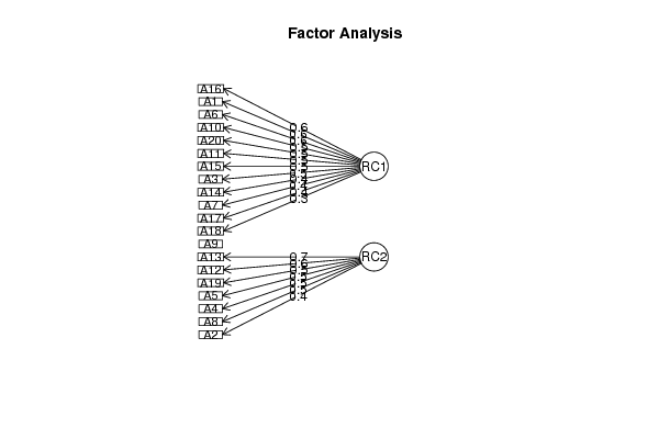
fit <- principal(y, nfactors=par1, rotate='varimax')
fit
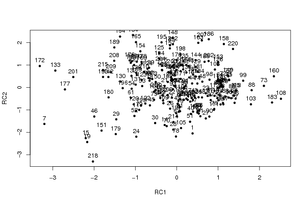
fs <- factor.scores(y,fit)
fs
bitmap(file='test1.png')
fa.diagram(fit)
dev.off()
bitmap(file='test2.png')
plot(fs,pch=20)
text(fs,labels=rownames(y),pos=3)
dev.off()
load(file='createtable')
a<-table.start()
a<-table.row.start(a)
a<-table.element(a,'Rotated Factor Loadings',par1+1,TRUE)
a<-table.row.end(a)
a<-table.row.start(a)
a<-table.element(a,'Variables',1,TRUE)
for (i in 1:par1) {
a<-table.element(a,paste('Factor',i,sep=''),1,TRUE)
}
a<-table.row.end(a)
for (j in 1:length(fit$loadings[,1])) {
a<-table.row.start(a)
a<-table.element(a,rownames(fit$loadings)[j],header=TRUE)
for (i in 1:par1) {
a<-table.element(a,round(fit$loadings[j,i],3))
}
a<-table.row.end(a)
}
a<-table.end(a)
table.save(a,file='mytable.tab')