Free Statistics
of Irreproducible Research!
Description of Statistical Computation | |||||||||||||||||||||
|---|---|---|---|---|---|---|---|---|---|---|---|---|---|---|---|---|---|---|---|---|---|
| Author's title | |||||||||||||||||||||
| Author | *Unverified author* | ||||||||||||||||||||
| R Software Module | rwasp_sdplot.wasp | ||||||||||||||||||||
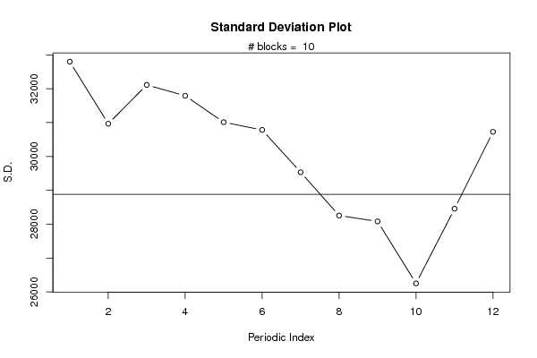
| Title produced by software | Standard Deviation Plot | ||||||||||||||||||||
| Date of computation | Wed, 08 Aug 2012 05:00:37 -0400 | ||||||||||||||||||||
| Cite this page as follows | Statistical Computations at FreeStatistics.org, Office for Research Development and Education, URL https://freestatistics.org/blog/index.php?v=date/2012/Aug/08/t1344416470m3x5j6v0rxow56o.htm/, Retrieved Fri, 03 May 2024 19:16:08 +0000 | ||||||||||||||||||||
| Statistical Computations at FreeStatistics.org, Office for Research Development and Education, URL https://freestatistics.org/blog/index.php?pk=169096, Retrieved Fri, 03 May 2024 19:16:08 +0000 | |||||||||||||||||||||
| QR Codes: | |||||||||||||||||||||
|
| |||||||||||||||||||||
| Original text written by user: | |||||||||||||||||||||
| IsPrivate? | No (this computation is public) | ||||||||||||||||||||
| User-defined keywords | Van der Smissen Britt | ||||||||||||||||||||
| Estimated Impact | 118 | ||||||||||||||||||||
Tree of Dependent Computations | |||||||||||||||||||||
| Family? (F = Feedback message, R = changed R code, M = changed R Module, P = changed Parameters, D = changed Data) | |||||||||||||||||||||
| - [Univariate Data Series] [Tijdreeks A-Stap 1] [2012-08-07 06:32:31] [e7a19f46406e1c79b79b562d86e5e00b] - RMP [Histogram] [Tijdreeks A-Stap 3] [2012-08-07 06:54:24] [e7a19f46406e1c79b79b562d86e5e00b] - RMP [Standard Deviation Plot] [Tijdreeks A-Stap 23] [2012-08-08 09:00:37] [b3616d670e39c9c081ac68ec1f5d1a32] [Current] | |||||||||||||||||||||
| Feedback Forum | |||||||||||||||||||||
Post a new message | |||||||||||||||||||||
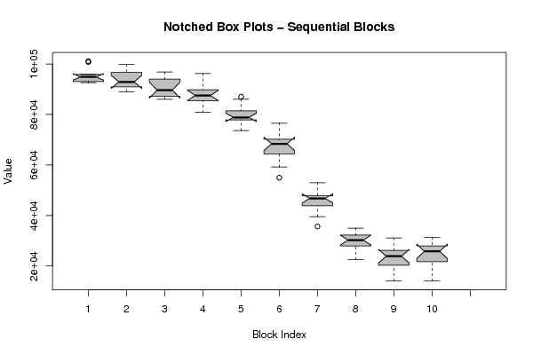
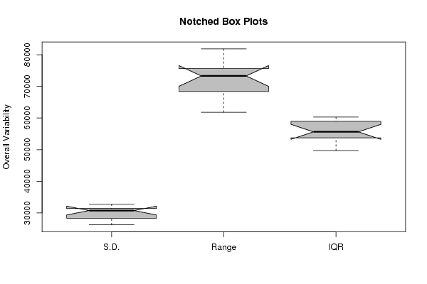
Dataset | |||||||||||||||||||||
| Dataseries X: | |||||||||||||||||||||
95870 95523 95208 94541 101097 100781 95870 92581 92928 92928 93244 93910 93559 96190 97172 96190 99799 97488 92261 90964 90964 91599 89004 90964 89319 90964 93559 94541 96852 95870 89981 87670 86692 87670 86057 86692 84728 88021 89635 89981 96190 96190 88021 86057 86057 87039 82764 80799 78524 79186 82133 79821 86057 87039 80799 78524 77221 78524 74910 73613 68390 69688 70004 70355 76559 75893 68390 65097 63799 65444 59208 54964 47115 47777 47777 47115 52684 53004 46448 45151 42524 46133 39577 35653 28146 29764 27800 28462 33373 34355 31093 30742 30742 35017 27484 22573 14058 20929 19946 20293 28146 27164 23555 25204 25204 31093 24222 20293 14058 22258 21595 21911 28782 28146 25835 26186 27800 31409 25835 21275 | |||||||||||||||||||||
Tables (Output of Computation) | |||||||||||||||||||||
| |||||||||||||||||||||
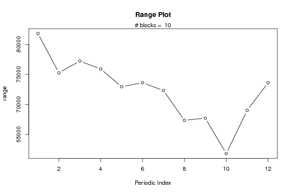
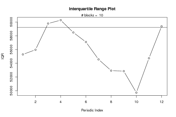
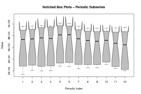
Figures (Output of Computation) | |||||||||||||||||||||
Input Parameters & R Code | |||||||||||||||||||||
| Parameters (Session): | |||||||||||||||||||||
| Parameters (R input): | |||||||||||||||||||||
| par1 = 12 ; | |||||||||||||||||||||
| R code (references can be found in the software module): | |||||||||||||||||||||
par1 <- '12' | |||||||||||||||||||||