Free Statistics
of Irreproducible Research!
Description of Statistical Computation | |||||||||||||||||||||||||||||||||||||||||||||||||
|---|---|---|---|---|---|---|---|---|---|---|---|---|---|---|---|---|---|---|---|---|---|---|---|---|---|---|---|---|---|---|---|---|---|---|---|---|---|---|---|---|---|---|---|---|---|---|---|---|---|
| Author's title | |||||||||||||||||||||||||||||||||||||||||||||||||
| Author | *The author of this computation has been verified* | ||||||||||||||||||||||||||||||||||||||||||||||||
| R Software Module | rwasp_tukeylambda.wasp | ||||||||||||||||||||||||||||||||||||||||||||||||
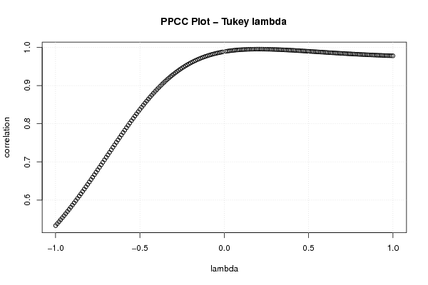
| Title produced by software | Tukey lambda PPCC Plot | ||||||||||||||||||||||||||||||||||||||||||||||||
| Date of computation | Thu, 30 Aug 2012 11:23:20 -0400 | ||||||||||||||||||||||||||||||||||||||||||||||||
| Cite this page as follows | Statistical Computations at FreeStatistics.org, Office for Research Development and Education, URL https://freestatistics.org/blog/index.php?v=date/2012/Aug/30/t13463402262epi45ymkjdzdpo.htm/, Retrieved Mon, 07 Jul 2025 05:21:18 +0000 | ||||||||||||||||||||||||||||||||||||||||||||||||
| Statistical Computations at FreeStatistics.org, Office for Research Development and Education, URL https://freestatistics.org/blog/index.php?pk=169603, Retrieved Mon, 07 Jul 2025 05:21:18 +0000 | |||||||||||||||||||||||||||||||||||||||||||||||||
| QR Codes: | |||||||||||||||||||||||||||||||||||||||||||||||||
|
| |||||||||||||||||||||||||||||||||||||||||||||||||
| Original text written by user: | |||||||||||||||||||||||||||||||||||||||||||||||||
| IsPrivate? | No (this computation is public) | ||||||||||||||||||||||||||||||||||||||||||||||||
| User-defined keywords | |||||||||||||||||||||||||||||||||||||||||||||||||
| Estimated Impact | 251 | ||||||||||||||||||||||||||||||||||||||||||||||||
Tree of Dependent Computations | |||||||||||||||||||||||||||||||||||||||||||||||||
| Family? (F = Feedback message, R = changed R code, M = changed R Module, P = changed Parameters, D = changed Data) | |||||||||||||||||||||||||||||||||||||||||||||||||
| - [Univariate Data Series] [] [2008-12-14 11:54:22] [d2d412c7f4d35ffbf5ee5ee89db327d4] - RMP [(Partial) Autocorrelation Function] [] [2011-12-06 20:17:24] [b98453cac15ba1066b407e146608df68] - RMPD [Tukey lambda PPCC Plot] [Tukey Lamda ] [2012-08-30 15:23:20] [c53b4e73f301bc561a9fa0b8f84a7890] [Current] | |||||||||||||||||||||||||||||||||||||||||||||||||
| Feedback Forum | |||||||||||||||||||||||||||||||||||||||||||||||||
Post a new message | |||||||||||||||||||||||||||||||||||||||||||||||||
Dataset | |||||||||||||||||||||||||||||||||||||||||||||||||
| Dataseries X: | |||||||||||||||||||||||||||||||||||||||||||||||||
293403 277108 264020 260646 246100 244051 241329 234730 234509 233482 233406 228548 223914 223696 223004 213765 210554 202204 199512 195304 191467 191381 191276 190410 188967 188780 185139 185039 184217 181853 181379 181344 179562 178863 178140 176789 176460 175877 175568 174107 173587 173260 172684 167845 167131 167105 166790 164767 162810 162336 161678 158980 157250 156833 155383 154991 154730 151503 146455 143937 142339 142146 142141 142069 141933 139350 139144 137793 136911 136548 135171 134043 131876 131122 130539 130533 130232 129100 128655 128066 127619 127324 126683 126681 125971 125366 122433 121135 119291 118958 118807 118372 116900 116775 115199 114928 114397 113337 111664 108715 107342 107335 106539 105615 105410 105324 103012 102531 101324 100885 100672 99946 99768 99246 98599 98030 94763 93340 93125 91185 90961 90938 89318 88817 84944 84572 84256 80953 78800 78776 75812 75426 74398 74112 73567 69471 68948 67746 67507 65029 64320 61857 61499 50999 46660 43287 38214 35523 32750 31414 24188 22938 21054 17547 14688 7199 969 455 203 98 0 0 0 0 | |||||||||||||||||||||||||||||||||||||||||||||||||
Tables (Output of Computation) | |||||||||||||||||||||||||||||||||||||||||||||||||
| |||||||||||||||||||||||||||||||||||||||||||||||||
Figures (Output of Computation) | |||||||||||||||||||||||||||||||||||||||||||||||||
Input Parameters & R Code | |||||||||||||||||||||||||||||||||||||||||||||||||
| Parameters (Session): | |||||||||||||||||||||||||||||||||||||||||||||||||
| par1 = 8 ; par2 = 0 ; | |||||||||||||||||||||||||||||||||||||||||||||||||
| Parameters (R input): | |||||||||||||||||||||||||||||||||||||||||||||||||
| R code (references can be found in the software module): | |||||||||||||||||||||||||||||||||||||||||||||||||
gp <- function(lambda, p) | |||||||||||||||||||||||||||||||||||||||||||||||||