Free Statistics
of Irreproducible Research!
Description of Statistical Computation | ||||||||||||||||||||||||||||||
|---|---|---|---|---|---|---|---|---|---|---|---|---|---|---|---|---|---|---|---|---|---|---|---|---|---|---|---|---|---|---|
| Author's title | ||||||||||||||||||||||||||||||
| Author | *The author of this computation has been verified* | |||||||||||||||||||||||||||||
| R Software Module | rwasp_Distributional Plots.wasp | |||||||||||||||||||||||||||||
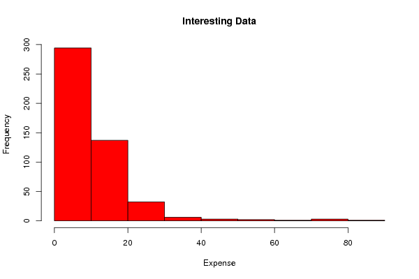
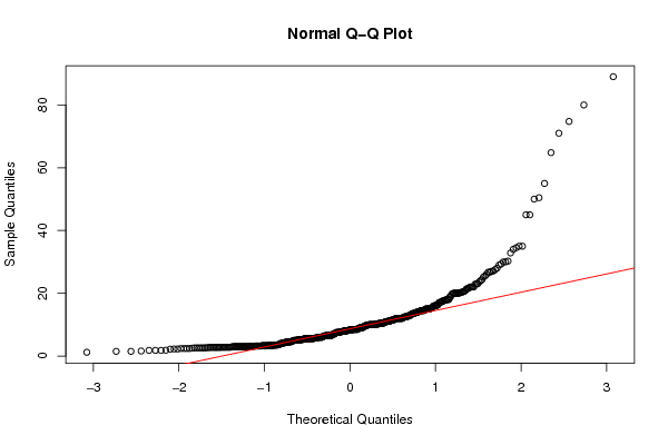
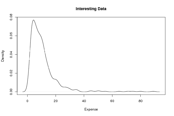
| Title produced by software | Histogram, QQplot and Density | |||||||||||||||||||||||||||||
| Date of computation | Mon, 02 Jul 2012 14:17:17 -0400 | |||||||||||||||||||||||||||||
| Cite this page as follows | Statistical Computations at FreeStatistics.org, Office for Research Development and Education, URL https://freestatistics.org/blog/index.php?v=date/2012/Jul/02/t1341253430452wpvqs1cwnho9.htm/, Retrieved Sat, 27 Apr 2024 20:15:04 +0000 | |||||||||||||||||||||||||||||
| Statistical Computations at FreeStatistics.org, Office for Research Development and Education, URL https://freestatistics.org/blog/index.php?pk=168759, Retrieved Sat, 27 Apr 2024 20:15:04 +0000 | ||||||||||||||||||||||||||||||
| QR Codes: | ||||||||||||||||||||||||||||||
|
| ||||||||||||||||||||||||||||||
| Original text written by user: | ||||||||||||||||||||||||||||||
| IsPrivate? | No (this computation is public) | |||||||||||||||||||||||||||||
| User-defined keywords | ||||||||||||||||||||||||||||||
| Estimated Impact | 212 | |||||||||||||||||||||||||||||
Tree of Dependent Computations | ||||||||||||||||||||||||||||||
| Family? (F = Feedback message, R = changed R code, M = changed R Module, P = changed Parameters, D = changed Data) | ||||||||||||||||||||||||||||||
| - [Histogram, QQplot and Density] [Possible Week 1 D...] [2012-07-02 18:17:17] [a9208f4f8d3b118336aae915785f2bd9] [Current] - R P [Histogram, QQplot and Density] [expense data with...] [2012-07-04 10:21:33] [98fd0e87c3eb04e0cc2efde01dbafab6] - R PD [Histogram, QQplot and Density] [Log(expense data)] [2012-07-04 10:24:16] [98fd0e87c3eb04e0cc2efde01dbafab6] - R D [Histogram, QQplot and Density] [Pub data Jan 2013] [2013-01-08 15:43:18] [74be16979710d4c4e7c6647856088456] | ||||||||||||||||||||||||||||||
| Feedback Forum | ||||||||||||||||||||||||||||||
Post a new message | ||||||||||||||||||||||||||||||
Dataset | ||||||||||||||||||||||||||||||
| Dataseries X: | ||||||||||||||||||||||||||||||
6.6 4.2 5 26.7 6.5 3.2 8.1 11.3 5 5 27.1 5.4 13.5 6.5 8.25 5.6 12.5 10.4 10.5 13.5 10.4 5.5 12 11.2 12.5 80 3.2 5.6 16.2 24 10 20.5 10.5 14.5 74.74 11 14.5 5.5 12 7.2 5.2 3.2 5.5 18 28 2.6 2.6 5.2 7.7 5.3 13.2 21.5 4.6 5.6 4.5 11.97 7.8 13.8 15.05 17.8 15 30 8 7.8 5.6 9.5 10.4 7.6 8.8 10.4 10.8 20 10.4 22 3.6 11.5 7.5 8.2 4.2 3.2 10.5 20 4.2 8.5 10.2 7 3.5 10 3.4 3.2 6.4 7.8 12.6 2.4 13 24.3 3.4 2.6 3.4 5 3.4 8.4 5.2 10.6 10 7.8 5.8 5.6 5.8 6.4 12.2 3.05 22 16 2.8 5.5 3.2 8 17.9 5.2 8.5 5.5 8.2 21.6 5.5 8.5 27.54 7.3 5.2 5.2 29.33 20 16 18.85 4.2 8.5 8.5 14 8.2 5.58 9.8 5.2 4.4 20 8.4 10.4 8 14.4 6.6 18 11 12 15.8 12.5 20.58 35 12.5 13 13.59 7.95 7.95 7.5 3.61 9.6 17.1 8.5 6 6 45 2.75 34 2.7 4.5 12 13.5 14.5 5.5 11.55 50 8.5 8.5 7.5 13.5 5.5 7.2 5.5 15 5.7 2.75 12.75 2.6 5.5 2.6 4.4 14.6 10 45 2.65 26 10.5 22 35 16.1 14 7 11.5 11.15 34.5 4 5.5 10.2 8.4 7.5 2.8 6.5 27 11 3.2 14.3 7.5 14.5 2.75 8.8 12 23 5.65 11.8 5.7 11.15 19.5 2.75 17 14.05 2.75 8.25 20.3 2.75 2.75 8.4 13 12 1.8 7.84 4.5 5.72 16.4 8.5 6 3 5.8 11.6 5.5 16.1 3.5 15 3 12 3 12.65 12 8.8 11.98 6 9 18 10.8 6 9 23 8.48 6.4 6.6 13.8 64.8 10 4 10 2.8 20 3 1.8 9 8 6.9 12 1.8 3 10 20.9 12.4 3 10.8 3 3 9 13.8 6 17.2 3 3 18.8 9 10 4 8 11.5 14.4 11 17.5 3.3 21.4 6.6 6.6 9.9 6.6 23.6 6 11 6 15 3.2 15 10 9 3.3 2.85 9.9 6.4 9.8 9.2 3.3 5.6 9.6 2.6 12 15.1 2.8 11.2 3.15 2.8 10 5 15.3 20 5 12.6 6.6 3.3 9.9 55 3.3 4.5 22 2.25 4.9 5 12.3 25.5 10 10.5 2.8 29 8.4 14 9 3.3 3.3 7 9 20.35 2.25 10 26.7 3.15 3.15 17.15 3.15 5.7 9.9 15.2 3 12.9 2.8 10.2 10 3.8 1.85 32.85 9.25 25.15 5.25 22.85 6 3 10.05 15.5 6.6 7.8 3.6 9.6 3 3.3 15 7.5 4.4 14.2 89 20 4.8 6.15 3.4 6.6 30.25 10.2 12 3 1.5 3.5 3.5 2.8 3.5 1.6 7.5 6.5 6 2.4 71 16.1 1.5 2.5 5.3 2.4 11.4 3.1 3.1 12 17.79 3 8 14.5 7.5 4 3.3 11.15 10.2 8.5 9.45 19.8 3.5 10.05 3.35 3.4 2.2 17.5 6.5 4.5 10.2 6.25 1.2 20.2 4.45 4.45 11.6 6.6 8.1 5.2 17.6 8.2 4.6 3 3 30 8.4 50.45 3.4 2.4 5.5 4.75 6.9 | ||||||||||||||||||||||||||||||
Tables (Output of Computation) | ||||||||||||||||||||||||||||||
| ||||||||||||||||||||||||||||||
Figures (Output of Computation) | ||||||||||||||||||||||||||||||
Input Parameters & R Code | ||||||||||||||||||||||||||||||
| Parameters (Session): | ||||||||||||||||||||||||||||||
| par1 = 10 ; | ||||||||||||||||||||||||||||||
| Parameters (R input): | ||||||||||||||||||||||||||||||
| par1 = 10 ; | ||||||||||||||||||||||||||||||
| R code (references can be found in the software module): | ||||||||||||||||||||||||||||||
par1 <- '10' | ||||||||||||||||||||||||||||||