Free Statistics

of Irreproducible Research!

Author's title

Author*The author of this computation has been verified*
R Software Modulerwasp_regression_trees1dm.wasp
Title produced by softwareRecursive Partitioning (Regression Trees)
Date of computationTue, 01 May 2012 07:42:26 -0400
Cite this page as followsStatistical Computations at FreeStatistics.org, Office for Research Development and Education, URL https://freestatistics.org/blog/index.php?v=date/2012/May/01/t1335872692qn2dnfetyxgzp3f.htm/, Retrieved Sat, 04 May 2024 06:19:25 +0000
Statistical Computations at FreeStatistics.org, Office for Research Development and Education, URL https://freestatistics.org/blog/index.php?pk=165463, Retrieved Sat, 04 May 2024 06:19:25 +0000
QR Codes:

Original text written by user:
IsPrivate?No (this computation is public)
User-defined keywords
Estimated Impact101
Family? (F = Feedback message, R = changed R code, M = changed R Module, P = changed Parameters, D = changed Data)
-       [Recursive Partitioning (Regression Trees)] [] [2012-05-01 11:42:26] [05300ca098a536dd63793e3fbb62faf1] [Current]
Feedback Forum

Post a new message


Summary of computational transaction
Raw Inputview raw input (R code)
Raw Outputview raw output of R engine
Computing time6 seconds
R Server'Gwilym Jenkins' @ jenkins.wessa.net

\begin{tabular}{lllllllll}
\hline
Summary of computational transaction \tabularnewline
Raw Input & view raw input (R code)  \tabularnewline
Raw Output & view raw output of R engine  \tabularnewline
Computing time & 6 seconds \tabularnewline
R Server & 'Gwilym Jenkins' @ jenkins.wessa.net \tabularnewline
\hline
\end{tabular}
%Source: https://freestatistics.org/blog/index.php?pk=165463&T=0

[TABLE]
[ROW][C]Summary of computational transaction[/C][/ROW]
[ROW][C]Raw Input[/C][C]view raw input (R code) [/C][/ROW]
[ROW][C]Raw Output[/C][C]view raw output of R engine [/C][/ROW]
[ROW][C]Computing time[/C][C]6 seconds[/C][/ROW]
[ROW][C]R Server[/C][C]'Gwilym Jenkins' @ jenkins.wessa.net[/C][/ROW]
[/TABLE]
Source: https://freestatistics.org/blog/index.php?pk=165463&T=0

Globally Unique Identifier (entire table): ba.freestatistics.org/blog/index.php?pk=165463&T=0

As an alternative you can also use a QR Code:  

The GUIDs for individual cells are displayed in the table below:

Summary of computational transaction
Raw Inputview raw input (R code)
Raw Outputview raw output of R engine
Computing time6 seconds
R Server'Gwilym Jenkins' @ jenkins.wessa.net


Goodness of Fit
Correlation0.5538
R-squared0.3067
RMSE2.9196

\begin{tabular}{lllllllll}
\hline
Goodness of Fit \tabularnewline
Correlation & 0.5538 \tabularnewline
R-squared & 0.3067 \tabularnewline
RMSE & 2.9196 \tabularnewline
\hline
\end{tabular}
%Source: https://freestatistics.org/blog/index.php?pk=165463&T=1

[TABLE]
[ROW][C]Goodness of Fit[/C][/ROW]
[ROW][C]Correlation[/C][C]0.5538[/C][/ROW]
[ROW][C]R-squared[/C][C]0.3067[/C][/ROW]
[ROW][C]RMSE[/C][C]2.9196[/C][/ROW]
[/TABLE]
Source: https://freestatistics.org/blog/index.php?pk=165463&T=1

Globally Unique Identifier (entire table): ba.freestatistics.org/blog/index.php?pk=165463&T=1

As an alternative you can also use a QR Code:  

The GUIDs for individual cells are displayed in the table below:

Goodness of Fit
Correlation0.5538
R-squared0.3067
RMSE2.9196


Actuals, Predictions, and Residuals
#ActualsForecastsResiduals
14239.16666666666672.83333333333334
23839.1666666666667-1.16666666666666
33735.17241379310341.82758620689656
43735.17241379310341.82758620689656
53835.17241379310342.82758620689656
64139.16666666666671.83333333333334
73839.1666666666667-1.16666666666666
84339.16666666666673.83333333333334
93535.1724137931034-0.172413793103445
103735.17241379310341.82758620689656
113235.1724137931034-3.17241379310344
123735.17241379310341.82758620689656
133035.1724137931034-5.17241379310344
143535.1724137931034-0.172413793103445
153839.1666666666667-1.16666666666666
163235.1724137931034-3.17241379310344
173635.17241379310340.827586206896555
183635.17241379310340.827586206896555
193735.17241379310341.82758620689656
203539.1666666666667-4.16666666666666
214035.17241379310344.82758620689656
223435.1724137931034-1.17241379310344
233935.17241379310343.82758620689656
243635.17241379310340.827586206896555
253535.1724137931034-0.172413793103445
263639.1666666666667-3.16666666666666
272635.1724137931034-9.17241379310344
283539.1666666666667-4.16666666666666
293635.17241379310340.827586206896555
303435.1724137931034-1.17241379310344
313535.1724137931034-0.172413793103445
323235.1724137931034-3.17241379310344
333835.17241379310342.82758620689656
343735.17241379310341.82758620689656
353635.17241379310340.827586206896555
364039.16666666666670.833333333333336
374539.16666666666675.83333333333334
384239.16666666666672.83333333333334
393939.1666666666667-0.166666666666664
403235.1724137931034-3.17241379310344
413839.1666666666667-1.16666666666666
424139.16666666666671.83333333333334
433635.17241379310340.827586206896555
443535.1724137931034-0.172413793103445
453939.1666666666667-0.166666666666664
464239.16666666666672.83333333333334
473339.1666666666667-6.16666666666666

\begin{tabular}{lllllllll}
\hline
Actuals, Predictions, and Residuals \tabularnewline
# & Actuals & Forecasts & Residuals \tabularnewline
1 & 42 & 39.1666666666667 & 2.83333333333334 \tabularnewline
2 & 38 & 39.1666666666667 & -1.16666666666666 \tabularnewline
3 & 37 & 35.1724137931034 & 1.82758620689656 \tabularnewline
4 & 37 & 35.1724137931034 & 1.82758620689656 \tabularnewline
5 & 38 & 35.1724137931034 & 2.82758620689656 \tabularnewline
6 & 41 & 39.1666666666667 & 1.83333333333334 \tabularnewline
7 & 38 & 39.1666666666667 & -1.16666666666666 \tabularnewline
8 & 43 & 39.1666666666667 & 3.83333333333334 \tabularnewline
9 & 35 & 35.1724137931034 & -0.172413793103445 \tabularnewline
10 & 37 & 35.1724137931034 & 1.82758620689656 \tabularnewline
11 & 32 & 35.1724137931034 & -3.17241379310344 \tabularnewline
12 & 37 & 35.1724137931034 & 1.82758620689656 \tabularnewline
13 & 30 & 35.1724137931034 & -5.17241379310344 \tabularnewline
14 & 35 & 35.1724137931034 & -0.172413793103445 \tabularnewline
15 & 38 & 39.1666666666667 & -1.16666666666666 \tabularnewline
16 & 32 & 35.1724137931034 & -3.17241379310344 \tabularnewline
17 & 36 & 35.1724137931034 & 0.827586206896555 \tabularnewline
18 & 36 & 35.1724137931034 & 0.827586206896555 \tabularnewline
19 & 37 & 35.1724137931034 & 1.82758620689656 \tabularnewline
20 & 35 & 39.1666666666667 & -4.16666666666666 \tabularnewline
21 & 40 & 35.1724137931034 & 4.82758620689656 \tabularnewline
22 & 34 & 35.1724137931034 & -1.17241379310344 \tabularnewline
23 & 39 & 35.1724137931034 & 3.82758620689656 \tabularnewline
24 & 36 & 35.1724137931034 & 0.827586206896555 \tabularnewline
25 & 35 & 35.1724137931034 & -0.172413793103445 \tabularnewline
26 & 36 & 39.1666666666667 & -3.16666666666666 \tabularnewline
27 & 26 & 35.1724137931034 & -9.17241379310344 \tabularnewline
28 & 35 & 39.1666666666667 & -4.16666666666666 \tabularnewline
29 & 36 & 35.1724137931034 & 0.827586206896555 \tabularnewline
30 & 34 & 35.1724137931034 & -1.17241379310344 \tabularnewline
31 & 35 & 35.1724137931034 & -0.172413793103445 \tabularnewline
32 & 32 & 35.1724137931034 & -3.17241379310344 \tabularnewline
33 & 38 & 35.1724137931034 & 2.82758620689656 \tabularnewline
34 & 37 & 35.1724137931034 & 1.82758620689656 \tabularnewline
35 & 36 & 35.1724137931034 & 0.827586206896555 \tabularnewline
36 & 40 & 39.1666666666667 & 0.833333333333336 \tabularnewline
37 & 45 & 39.1666666666667 & 5.83333333333334 \tabularnewline
38 & 42 & 39.1666666666667 & 2.83333333333334 \tabularnewline
39 & 39 & 39.1666666666667 & -0.166666666666664 \tabularnewline
40 & 32 & 35.1724137931034 & -3.17241379310344 \tabularnewline
41 & 38 & 39.1666666666667 & -1.16666666666666 \tabularnewline
42 & 41 & 39.1666666666667 & 1.83333333333334 \tabularnewline
43 & 36 & 35.1724137931034 & 0.827586206896555 \tabularnewline
44 & 35 & 35.1724137931034 & -0.172413793103445 \tabularnewline
45 & 39 & 39.1666666666667 & -0.166666666666664 \tabularnewline
46 & 42 & 39.1666666666667 & 2.83333333333334 \tabularnewline
47 & 33 & 39.1666666666667 & -6.16666666666666 \tabularnewline
\hline
\end{tabular}
%Source: https://freestatistics.org/blog/index.php?pk=165463&T=2

[TABLE]
[ROW][C]Actuals, Predictions, and Residuals[/C][/ROW]
[ROW][C]#[/C][C]Actuals[/C][C]Forecasts[/C][C]Residuals[/C][/ROW]
[ROW][C]1[/C][C]42[/C][C]39.1666666666667[/C][C]2.83333333333334[/C][/ROW]
[ROW][C]2[/C][C]38[/C][C]39.1666666666667[/C][C]-1.16666666666666[/C][/ROW]
[ROW][C]3[/C][C]37[/C][C]35.1724137931034[/C][C]1.82758620689656[/C][/ROW]
[ROW][C]4[/C][C]37[/C][C]35.1724137931034[/C][C]1.82758620689656[/C][/ROW]
[ROW][C]5[/C][C]38[/C][C]35.1724137931034[/C][C]2.82758620689656[/C][/ROW]
[ROW][C]6[/C][C]41[/C][C]39.1666666666667[/C][C]1.83333333333334[/C][/ROW]
[ROW][C]7[/C][C]38[/C][C]39.1666666666667[/C][C]-1.16666666666666[/C][/ROW]
[ROW][C]8[/C][C]43[/C][C]39.1666666666667[/C][C]3.83333333333334[/C][/ROW]
[ROW][C]9[/C][C]35[/C][C]35.1724137931034[/C][C]-0.172413793103445[/C][/ROW]
[ROW][C]10[/C][C]37[/C][C]35.1724137931034[/C][C]1.82758620689656[/C][/ROW]
[ROW][C]11[/C][C]32[/C][C]35.1724137931034[/C][C]-3.17241379310344[/C][/ROW]
[ROW][C]12[/C][C]37[/C][C]35.1724137931034[/C][C]1.82758620689656[/C][/ROW]
[ROW][C]13[/C][C]30[/C][C]35.1724137931034[/C][C]-5.17241379310344[/C][/ROW]
[ROW][C]14[/C][C]35[/C][C]35.1724137931034[/C][C]-0.172413793103445[/C][/ROW]
[ROW][C]15[/C][C]38[/C][C]39.1666666666667[/C][C]-1.16666666666666[/C][/ROW]
[ROW][C]16[/C][C]32[/C][C]35.1724137931034[/C][C]-3.17241379310344[/C][/ROW]
[ROW][C]17[/C][C]36[/C][C]35.1724137931034[/C][C]0.827586206896555[/C][/ROW]
[ROW][C]18[/C][C]36[/C][C]35.1724137931034[/C][C]0.827586206896555[/C][/ROW]
[ROW][C]19[/C][C]37[/C][C]35.1724137931034[/C][C]1.82758620689656[/C][/ROW]
[ROW][C]20[/C][C]35[/C][C]39.1666666666667[/C][C]-4.16666666666666[/C][/ROW]
[ROW][C]21[/C][C]40[/C][C]35.1724137931034[/C][C]4.82758620689656[/C][/ROW]
[ROW][C]22[/C][C]34[/C][C]35.1724137931034[/C][C]-1.17241379310344[/C][/ROW]
[ROW][C]23[/C][C]39[/C][C]35.1724137931034[/C][C]3.82758620689656[/C][/ROW]
[ROW][C]24[/C][C]36[/C][C]35.1724137931034[/C][C]0.827586206896555[/C][/ROW]
[ROW][C]25[/C][C]35[/C][C]35.1724137931034[/C][C]-0.172413793103445[/C][/ROW]
[ROW][C]26[/C][C]36[/C][C]39.1666666666667[/C][C]-3.16666666666666[/C][/ROW]
[ROW][C]27[/C][C]26[/C][C]35.1724137931034[/C][C]-9.17241379310344[/C][/ROW]
[ROW][C]28[/C][C]35[/C][C]39.1666666666667[/C][C]-4.16666666666666[/C][/ROW]
[ROW][C]29[/C][C]36[/C][C]35.1724137931034[/C][C]0.827586206896555[/C][/ROW]
[ROW][C]30[/C][C]34[/C][C]35.1724137931034[/C][C]-1.17241379310344[/C][/ROW]
[ROW][C]31[/C][C]35[/C][C]35.1724137931034[/C][C]-0.172413793103445[/C][/ROW]
[ROW][C]32[/C][C]32[/C][C]35.1724137931034[/C][C]-3.17241379310344[/C][/ROW]
[ROW][C]33[/C][C]38[/C][C]35.1724137931034[/C][C]2.82758620689656[/C][/ROW]
[ROW][C]34[/C][C]37[/C][C]35.1724137931034[/C][C]1.82758620689656[/C][/ROW]
[ROW][C]35[/C][C]36[/C][C]35.1724137931034[/C][C]0.827586206896555[/C][/ROW]
[ROW][C]36[/C][C]40[/C][C]39.1666666666667[/C][C]0.833333333333336[/C][/ROW]
[ROW][C]37[/C][C]45[/C][C]39.1666666666667[/C][C]5.83333333333334[/C][/ROW]
[ROW][C]38[/C][C]42[/C][C]39.1666666666667[/C][C]2.83333333333334[/C][/ROW]
[ROW][C]39[/C][C]39[/C][C]39.1666666666667[/C][C]-0.166666666666664[/C][/ROW]
[ROW][C]40[/C][C]32[/C][C]35.1724137931034[/C][C]-3.17241379310344[/C][/ROW]
[ROW][C]41[/C][C]38[/C][C]39.1666666666667[/C][C]-1.16666666666666[/C][/ROW]
[ROW][C]42[/C][C]41[/C][C]39.1666666666667[/C][C]1.83333333333334[/C][/ROW]
[ROW][C]43[/C][C]36[/C][C]35.1724137931034[/C][C]0.827586206896555[/C][/ROW]
[ROW][C]44[/C][C]35[/C][C]35.1724137931034[/C][C]-0.172413793103445[/C][/ROW]
[ROW][C]45[/C][C]39[/C][C]39.1666666666667[/C][C]-0.166666666666664[/C][/ROW]
[ROW][C]46[/C][C]42[/C][C]39.1666666666667[/C][C]2.83333333333334[/C][/ROW]
[ROW][C]47[/C][C]33[/C][C]39.1666666666667[/C][C]-6.16666666666666[/C][/ROW]
[/TABLE]
Source: https://freestatistics.org/blog/index.php?pk=165463&T=2

Globally Unique Identifier (entire table): ba.freestatistics.org/blog/index.php?pk=165463&T=2

As an alternative you can also use a QR Code:  

The GUIDs for individual cells are displayed in the table below:

Actuals, Predictions, and Residuals
#ActualsForecastsResiduals
14239.16666666666672.83333333333334
23839.1666666666667-1.16666666666666
33735.17241379310341.82758620689656
43735.17241379310341.82758620689656
53835.17241379310342.82758620689656
64139.16666666666671.83333333333334
73839.1666666666667-1.16666666666666
84339.16666666666673.83333333333334
93535.1724137931034-0.172413793103445
103735.17241379310341.82758620689656
113235.1724137931034-3.17241379310344
123735.17241379310341.82758620689656
133035.1724137931034-5.17241379310344
143535.1724137931034-0.172413793103445
153839.1666666666667-1.16666666666666
163235.1724137931034-3.17241379310344
173635.17241379310340.827586206896555
183635.17241379310340.827586206896555
193735.17241379310341.82758620689656
203539.1666666666667-4.16666666666666
214035.17241379310344.82758620689656
223435.1724137931034-1.17241379310344
233935.17241379310343.82758620689656
243635.17241379310340.827586206896555
253535.1724137931034-0.172413793103445
263639.1666666666667-3.16666666666666
272635.1724137931034-9.17241379310344
283539.1666666666667-4.16666666666666
293635.17241379310340.827586206896555
303435.1724137931034-1.17241379310344
313535.1724137931034-0.172413793103445
323235.1724137931034-3.17241379310344
333835.17241379310342.82758620689656
343735.17241379310341.82758620689656
353635.17241379310340.827586206896555
364039.16666666666670.833333333333336
374539.16666666666675.83333333333334
384239.16666666666672.83333333333334
393939.1666666666667-0.166666666666664
403235.1724137931034-3.17241379310344
413839.1666666666667-1.16666666666666
424139.16666666666671.83333333333334
433635.17241379310340.827586206896555
443535.1724137931034-0.172413793103445
453939.1666666666667-0.166666666666664
464239.16666666666672.83333333333334
473339.1666666666667-6.16666666666666


Parameters (Session):
par1 = 0 ; par2 = none ; par3 = 3 ; par4 = no ; par5 = female ; par6 = bachelor ; par7 = 1 ; par8 = ATTLES connected ; par9 = ATTLES connected ;
Parameters (R input):
par1 = 0 ; par2 = none ; par3 = 3 ; par4 = no ; par5 = female ; par6 = bachelor ; par7 = 1 ; par8 = ATTLES connected ; par9 = ATTLES connected ;
R code (references can be found in the software module):
library(party)
library(Hmisc)
par1 <- as.numeric(par1)
par3 <- as.numeric(par3)
x <- as.data.frame(read.table(file='https://automated.biganalytics.eu/download/utaut.csv',sep=',',header=T))
x$U25 <- 6-x$U25
if(par5 == 'female') x <- x[x$Gender==0,]
if(par5 == 'male') x <- x[x$Gender==1,]
if(par6 == 'prep') x <- x[x$Pop==1,]
if(par6 == 'bachelor') x <- x[x$Pop==0,]
if(par7 != 'all') {
x <- x[x$Year==as.numeric(par7),]
}
cAc <- with(x,cbind( A1, A2, A3, A4, A5, A6, A7, A8, A9,A10))
cAs <- with(x,cbind(A11,A12,A13,A14,A15,A16,A17,A18,A19,A20))
cA <- cbind(cAc,cAs)
cCa <- with(x,cbind(C1,C3,C5,C7, C9,C11,C13,C15,C17,C19,C21,C23,C25,C27,C29,C31,C33,C35,C37,C39,C41,C43,C45,C47))
cCp <- with(x,cbind(C2,C4,C6,C8,C10,C12,C14,C16,C18,C20,C22,C24,C26,C28,C30,C32,C34,C36,C38,C40,C42,C44,C46,C48))
cC <- cbind(cCa,cCp)
cU <- with(x,cbind(U1,U2,U3,U4,U5,U6,U7,U8,U9,U10,U11,U12,U13,U14,U15,U16,U17,U18,U19,U20,U21,U22,U23,U24,U25,U26,U27,U28,U29,U30,U31,U32,U33))
cE <- with(x,cbind(BC,NNZFG,MRT,AFL,LPM,LPC,W,WPA))
cX <- with(x,cbind(X1,X2,X3,X4,X5,X6,X7,X8,X9,X10,X11,X12,X13,X14,X15,X16,X17,X18))
if (par8=='ATTLES connected') x <- cAc
if (par8=='ATTLES separate') x <- cAs
if (par8=='ATTLES all') x <- cA
if (par8=='COLLES actuals') x <- cCa
if (par8=='COLLES preferred') x <- cCp
if (par8=='COLLES all') x <- cC
if (par8=='CSUQ') x <- cU
if (par8=='Learning Activities') x <- cE
if (par8=='Exam Items') x <- cX
if (par9=='ATTLES connected') y <- cAc
if (par9=='ATTLES separate') y <- cAs
if (par9=='ATTLES all') y <- cA
if (par9=='COLLES actuals') y <- cCa
if (par9=='COLLES preferred') y <- cCp
if (par9=='COLLES all') y <- cC
if (par9=='CSUQ') y <- cU
if (par9=='Learning Activities') y <- cE
if (par9=='Exam Items') y <- cX
if (par1==0) {
nr <- length(y[,1])
nc <- length(y[1,])
mysum <- array(0,dim=nr)
for(jjj in 1:nr) {
for(iii in 1:nc) {
mysum[jjj] = mysum[jjj] + y[jjj,iii]
}
}
y <- mysum
} else {
y <- y[,par1]
}
nx <- cbind(y,x)
colnames(nx) <- c('endo',colnames(x))
x <- nx
par1=1
ncol <- length(x[1,])
for (jjj in 1:ncol) {
x <- x[!is.na(x[,jjj]),]
}
x <- as.data.frame(x)
k <- length(x[1,])
n <- length(x[,1])
colnames(x)[par1]
x[,par1]
if (par2 == 'kmeans') {
cl <- kmeans(x[,par1], par3)
print(cl)
clm <- matrix(cbind(cl$centers,1:par3),ncol=2)
clm <- clm[sort.list(clm[,1]),]
for (i in 1:par3) {
cl$cluster[cl$cluster==clm[i,2]] <- paste('C',i,sep='')
}
cl$cluster <- as.factor(cl$cluster)
print(cl$cluster)
x[,par1] <- cl$cluster
}
if (par2 == 'quantiles') {
x[,par1] <- cut2(x[,par1],g=par3)
}
if (par2 == 'hclust') {
hc <- hclust(dist(x[,par1])^2, 'cen')
print(hc)
memb <- cutree(hc, k = par3)
dum <- c(mean(x[memb==1,par1]))
for (i in 2:par3) {
dum <- c(dum, mean(x[memb==i,par1]))
}
hcm <- matrix(cbind(dum,1:par3),ncol=2)
hcm <- hcm[sort.list(hcm[,1]),]
for (i in 1:par3) {
memb[memb==hcm[i,2]] <- paste('C',i,sep='')
}
memb <- as.factor(memb)
print(memb)
x[,par1] <- memb
}
if (par2=='equal') {
ed <- cut(as.numeric(x[,par1]),par3,labels=paste('C',1:par3,sep=''))
x[,par1] <- as.factor(ed)
}
table(x[,par1])
colnames(x)
colnames(x)[par1]
x[,par1]
if (par2 == 'none') {
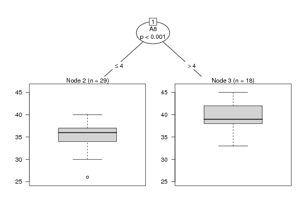
m <- ctree(as.formula(paste(colnames(x)[par1],' ~ .',sep='')),data = x)
}
load(file='createtable')
if (par2 != 'none') {
m <- ctree(as.formula(paste('as.factor(',colnames(x)[par1],') ~ .',sep='')),data = x)
if (par4=='yes') {
a<-table.start()
a<-table.row.start(a)
a<-table.element(a,'10-Fold Cross Validation',3+2*par3,TRUE)
a<-table.row.end(a)
a<-table.row.start(a)
a<-table.element(a,'',1,TRUE)
a<-table.element(a,'Prediction (training)',par3+1,TRUE)
a<-table.element(a,'Prediction (testing)',par3+1,TRUE)
a<-table.row.end(a)
a<-table.row.start(a)
a<-table.element(a,'Actual',1,TRUE)
for (jjj in 1:par3) a<-table.element(a,paste('C',jjj,sep=''),1,TRUE)
a<-table.element(a,'CV',1,TRUE)
for (jjj in 1:par3) a<-table.element(a,paste('C',jjj,sep=''),1,TRUE)
a<-table.element(a,'CV',1,TRUE)
a<-table.row.end(a)
for (i in 1:10) {
ind <- sample(2, nrow(x), replace=T, prob=c(0.9,0.1))
m.ct <- ctree(as.formula(paste('as.factor(',colnames(x)[par1],') ~ .',sep='')),data =x[ind==1,])
if (i==1) {
m.ct.i.pred <- predict(m.ct, newdata=x[ind==1,])
m.ct.i.actu <- x[ind==1,par1]
m.ct.x.pred <- predict(m.ct, newdata=x[ind==2,])
m.ct.x.actu <- x[ind==2,par1]
} else {
m.ct.i.pred <- c(m.ct.i.pred,predict(m.ct, newdata=x[ind==1,]))
m.ct.i.actu <- c(m.ct.i.actu,x[ind==1,par1])
m.ct.x.pred <- c(m.ct.x.pred,predict(m.ct, newdata=x[ind==2,]))
m.ct.x.actu <- c(m.ct.x.actu,x[ind==2,par1])
}
}
print(m.ct.i.tab <- table(m.ct.i.actu,m.ct.i.pred))
numer <- 0
for (i in 1:par3) {
print(m.ct.i.tab[i,i] / sum(m.ct.i.tab[i,]))
numer <- numer + m.ct.i.tab[i,i]
}
print(m.ct.i.cp <- numer / sum(m.ct.i.tab))
print(m.ct.x.tab <- table(m.ct.x.actu,m.ct.x.pred))
numer <- 0
for (i in 1:par3) {
print(m.ct.x.tab[i,i] / sum(m.ct.x.tab[i,]))
numer <- numer + m.ct.x.tab[i,i]
}
print(m.ct.x.cp <- numer / sum(m.ct.x.tab))
for (i in 1:par3) {
a<-table.row.start(a)
a<-table.element(a,paste('C',i,sep=''),1,TRUE)
for (jjj in 1:par3) a<-table.element(a,m.ct.i.tab[i,jjj])
a<-table.element(a,round(m.ct.i.tab[i,i]/sum(m.ct.i.tab[i,]),4))
for (jjj in 1:par3) a<-table.element(a,m.ct.x.tab[i,jjj])
a<-table.element(a,round(m.ct.x.tab[i,i]/sum(m.ct.x.tab[i,]),4))
a<-table.row.end(a)
}
a<-table.row.start(a)
a<-table.element(a,'Overall',1,TRUE)
for (jjj in 1:par3) a<-table.element(a,'-')
a<-table.element(a,round(m.ct.i.cp,4))
for (jjj in 1:par3) a<-table.element(a,'-')
a<-table.element(a,round(m.ct.x.cp,4))
a<-table.row.end(a)
a<-table.end(a)
table.save(a,file='mytable3.tab')
}
}
m
bitmap(file='test1.png')
plot(m)
dev.off()
bitmap(file='test1a.png')
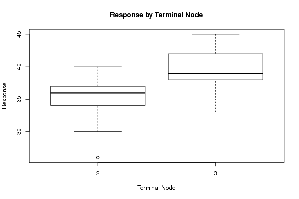
plot(x[,par1] ~ as.factor(where(m)),main='Response by Terminal Node',xlab='Terminal Node',ylab='Response')
dev.off()
if (par2 == 'none') {
forec <- predict(m)
result <- as.data.frame(cbind(x[,par1],forec,x[,par1]-forec))
colnames(result) <- c('Actuals','Forecasts','Residuals')
print(result)
}
if (par2 != 'none') {
print(cbind(as.factor(x[,par1]),predict(m)))
myt <- table(as.factor(x[,par1]),predict(m))
print(myt)
}
bitmap(file='test2.png')
if(par2=='none') {
op <- par(mfrow=c(2,2))
plot(density(result$Actuals),main='Kernel Density Plot of Actuals')
plot(density(result$Residuals),main='Kernel Density Plot of Residuals')
plot(result$Forecasts,result$Actuals,main='Actuals versus Predictions',xlab='Predictions',ylab='Actuals')
plot(density(result$Forecasts),main='Kernel Density Plot of Predictions')
par(op)
}
if(par2!='none') {
plot(myt,main='Confusion Matrix',xlab='Actual',ylab='Predicted')
}
dev.off()
if (par2 == 'none') {
detcoef <- cor(result$Forecasts,result$Actuals)
a<-table.start()
a<-table.row.start(a)
a<-table.element(a,'Goodness of Fit',2,TRUE)
a<-table.row.end(a)
a<-table.row.start(a)
a<-table.element(a,'Correlation',1,TRUE)
a<-table.element(a,round(detcoef,4))
a<-table.row.end(a)
a<-table.row.start(a)
a<-table.element(a,'R-squared',1,TRUE)
a<-table.element(a,round(detcoef*detcoef,4))
a<-table.row.end(a)
a<-table.row.start(a)
a<-table.element(a,'RMSE',1,TRUE)
a<-table.element(a,round(sqrt(mean((result$Residuals)^2)),4))
a<-table.row.end(a)
a<-table.end(a)
table.save(a,file='mytable1.tab')
a<-table.start()
a<-table.row.start(a)
a<-table.element(a,'Actuals, Predictions, and Residuals',4,TRUE)
a<-table.row.end(a)
a<-table.row.start(a)
a<-table.element(a,'#',header=TRUE)
a<-table.element(a,'Actuals',header=TRUE)
a<-table.element(a,'Forecasts',header=TRUE)
a<-table.element(a,'Residuals',header=TRUE)
a<-table.row.end(a)
for (i in 1:length(result$Actuals)) {
a<-table.row.start(a)
a<-table.element(a,i,header=TRUE)
a<-table.element(a,result$Actuals[i])
a<-table.element(a,result$Forecasts[i])
a<-table.element(a,result$Residuals[i])
a<-table.row.end(a)
}
a<-table.end(a)
table.save(a,file='mytable.tab')
}
if (par2 != 'none') {
a<-table.start()
a<-table.row.start(a)
a<-table.element(a,'Confusion Matrix (predicted in columns / actuals in rows)',par3+1,TRUE)
a<-table.row.end(a)
a<-table.row.start(a)
a<-table.element(a,'',1,TRUE)
for (i in 1:par3) {
a<-table.element(a,paste('C',i,sep=''),1,TRUE)
}
a<-table.row.end(a)
for (i in 1:par3) {
a<-table.row.start(a)
a<-table.element(a,paste('C',i,sep=''),1,TRUE)
for (j in 1:par3) {
a<-table.element(a,myt[i,j])
}
a<-table.row.end(a)
}
a<-table.end(a)
table.save(a,file='mytable2.tab')
}