Repository of Reproducible Computations

Free Statistics

of Irreproducible Research!

Author's title

Author

*Unverified author*

R Software Module

rwasp_bootstrapplot.wasp

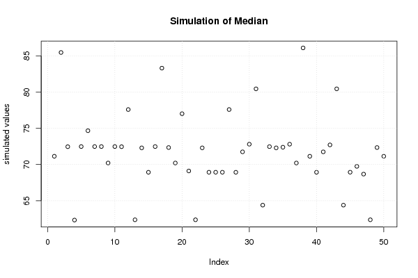
Title produced by software

Blocked Bootstrap Plot - Central Tendency

Date of computation

Wed, 02 May 2012 15:52:56 -0400

Cite this page as follows

Statistical Computations at FreeStatistics.org, Office for Research Development and Education, URL https://freestatistics.org/blog/index.php?v=date/2012/May/02/t13359884061uf4e8wl7g5m6qi.htm/, Retrieved Tue, 07 May 2024 11:53:54 +0000

Statistical Computations at FreeStatistics.org, Office for Research Development and Education, URL https://freestatistics.org/blog/index.php?pk=165991, Retrieved Tue, 07 May 2024 11:53:54 +0000

QR Codes:

Paste this QR Code to cite your computation.

Original text written by user:

IsPrivate?

No (this computation is public)

User-defined keywords

Estimated Impact

120

Family? (F = Feedback message, R = changed R code, M = changed R Module, P = changed Parameters, D = changed Data)

-     [Bootstrap Plot - Central Tendency] [Bootstrap Plot va...] [2012-05-02 19:39:36] [562ee1d5a96d07a2dc4978b28f7ac089]
- RMPD    [Blocked Bootstrap Plot - Central Tendency] [Blocked Bootstrap...] [2012-05-02 19:52:56] [1f07dfe249cf12c76d4857e2b59f088a] [Current]
- RMPD      [Variability] [spreidingsmaten m...] [2012-05-02 19:59:13] [562ee1d5a96d07a2dc4978b28f7ac089] 
- RMPD      [Standard Deviation Plot] [Standard Deviatio...] [2012-05-02 20:02:11] [562ee1d5a96d07a2dc4978b28f7ac089] 
-   PD        [Standard Deviation Plot] [] [2012-05-21 08:01:19] [314c90c95929b793e8a10c15bae12703] 
- RMPD        [Variability] [] [2012-05-21 08:13:49] [314c90c95929b793e8a10c15bae12703] 
-   PD        [Standard Deviation Plot] [] [2012-05-21 08:17:21] [314c90c95929b793e8a10c15bae12703] 
- RMPD        [Standard Deviation-Mean Plot] [] [2012-05-21 08:21:14] [314c90c95929b793e8a10c15bae12703] 
- RMPD        [Classical Decomposition] [] [2012-05-21 08:46:50] [314c90c95929b793e8a10c15bae12703] 
- RMPD        [Classical Decomposition] [] [2012-05-21 08:49:02] [314c90c95929b793e8a10c15bae12703] 
- RMPD        [Classical Decomposition] [] [2012-05-21 08:57:57] [314c90c95929b793e8a10c15bae12703] 
- RMPD        [Exponential Smoothing] [] [2012-05-21 09:05:57] [2f0f353a58a70fd7baf0f5141860d820] 
- RMPD        [Exponential Smoothing] [] [2012-05-21 09:12:08] [2f0f353a58a70fd7baf0f5141860d820] 
- RMPD      [Standard Deviation-Mean Plot] [Standard Deviatio...] [2012-05-02 20:04:42] [562ee1d5a96d07a2dc4978b28f7ac089] 
- RMP       [Variability] [Variability GSM g...] [2012-05-02 20:06:55] [562ee1d5a96d07a2dc4978b28f7ac089] 
- RMP       [Standard Deviation Plot] [Standard Deviatio...] [2012-05-02 20:08:34] [562ee1d5a96d07a2dc4978b28f7ac089] 
- RMPD      [Standard Deviation-Mean Plot] [Blocked Bootstrap...] [2012-05-02 20:10:39] [562ee1d5a96d07a2dc4978b28f7ac089] 

Feedback Forum

Post a new message

Dataseries X:

Download CSV

Histogram

Boxplots

Summary of computational transaction
Raw Input	view raw input (R code)
Raw Output	view raw output of R engine
Computing time	4 seconds
R Server	'Gwilym Jenkins' @ jenkins.wessa.net

\begin{tabular}{lllllllll}
\hline
Summary of computational transaction \tabularnewline
Raw Input & view raw input (R code)  \tabularnewline
Raw Output & view raw output of R engine  \tabularnewline
Computing time & 4 seconds \tabularnewline
R Server & 'Gwilym Jenkins' @ jenkins.wessa.net \tabularnewline
\hline
\end{tabular}
%Source: https://freestatistics.org/blog/index.php?pk=165991&T=0

[TABLE]
[ROW][C]Summary of computational transaction[/C][/ROW]
[ROW][C]Raw Input[/C][C]view raw input (R code) [/C][/ROW]
[ROW][C]Raw Output[/C][C]view raw output of R engine [/C][/ROW]
[ROW][C]Computing time[/C][C]4 seconds[/C][/ROW]
[ROW][C]R Server[/C][C]'Gwilym Jenkins' @ jenkins.wessa.net[/C][/ROW]
[/TABLE]
Source: https://freestatistics.org/blog/index.php?pk=165991&T=0

Globally Unique Identifier (entire table): ba.freestatistics.org/blog/index.php?pk=165991&T=0

As an alternative you can also use a QR Code:

The GUIDs for individual cells are displayed in the table below:

Summary of computational transaction
Raw Input	view raw input (R code)
Raw Output	view raw output of R engine
Computing time	4 seconds
R Server	'Gwilym Jenkins' @ jenkins.wessa.net

Estimation Results of Blocked Bootstrap
statistic	Q1	Estimate	Q3	S.D.	IQR
mean	71.2822916666667	73.2305	75.1834166666667	3.75113154688566	3.90112500000001
median	68.93625	71.75	72.48	5.22560191240576	3.54375
midrange	73.89875	75.415	75.415	3.34082130467882	1.51625

\begin{tabular}{lllllllll}
\hline
Estimation Results of Blocked Bootstrap \tabularnewline
statistic & Q1 & Estimate & Q3 & S.D. & IQR \tabularnewline
mean & 71.2822916666667 & 73.2305 & 75.1834166666667 & 3.75113154688566 & 3.90112500000001 \tabularnewline
median & 68.93625 & 71.75 & 72.48 & 5.22560191240576 & 3.54375 \tabularnewline
midrange & 73.89875 & 75.415 & 75.415 & 3.34082130467882 & 1.51625 \tabularnewline
\hline
\end{tabular}
%Source: https://freestatistics.org/blog/index.php?pk=165991&T=1

[TABLE]
[ROW][C]Estimation Results of Blocked Bootstrap[/C][/ROW]
[ROW][C]statistic[/C][C]Q1[/C][C]Estimate[/C][C]Q3[/C][C]S.D.[/C][C]IQR[/C][/ROW]
[ROW][C]mean[/C][C]71.2822916666667[/C][C]73.2305[/C][C]75.1834166666667[/C][C]3.75113154688566[/C][C]3.90112500000001[/C][/ROW]
[ROW][C]median[/C][C]68.93625[/C][C]71.75[/C][C]72.48[/C][C]5.22560191240576[/C][C]3.54375[/C][/ROW]
[ROW][C]midrange[/C][C]73.89875[/C][C]75.415[/C][C]75.415[/C][C]3.34082130467882[/C][C]1.51625[/C][/ROW]
[/TABLE]
Source: https://freestatistics.org/blog/index.php?pk=165991&T=1

Globally Unique Identifier (entire table): ba.freestatistics.org/blog/index.php?pk=165991&T=1

As an alternative you can also use a QR Code:

The GUIDs for individual cells are displayed in the table below:

Estimation Results of Blocked Bootstrap
statistic	Q1	Estimate	Q3	S.D.	IQR
mean	71.2822916666667	73.2305	75.1834166666667	3.75113154688566	3.90112500000001
median	68.93625	71.75	72.48	5.22560191240576	3.54375
midrange	73.89875	75.415	75.415	3.34082130467882	1.51625

Figure 1

PNG link

Postscript link

PDF link

Figure 2

PNG link

Postscript link

PDF link

Figure 3

PNG link

Postscript link

PDF link

Figure 4

PNG link

Postscript link

PDF link

Figure 5

PNG link

Postscript link

PDF link

Figure 6

PNG link

Postscript link

PDF link

Figure 7

PNG link

Postscript link

PDF link

Parameters (Session):

par1 = 50 ; par2 = 12 ;

Parameters (R input):

par1 = 50 ; par2 = 12 ;

R code (references can be found in the software module):

par1 <- as.numeric(par1)
par2 <- as.numeric(par2)
if (par1 < 10) par1 = 10
if (par1 > 5000) par1 = 5000
if (par2 < 3) par2 = 3
if (par2 > length(x)) par2 = length(x)
library(lattice)
library(boot)
boot.stat <- function(s)
{
s.mean <- mean(s)
s.median <- median(s)
s.midrange <- (max(s) + min(s)) / 2
c(s.mean, s.median, s.midrange)
}
(r <- tsboot(x, boot.stat, R=par1, l=12, sim='fixed'))
bitmap(file='plot1.png')
plot(r$t[,1],type='p',ylab='simulated values',main='Simulation of Mean')
grid()
dev.off()
bitmap(file='plot2.png')
plot(r$t[,2],type='p',ylab='simulated values',main='Simulation of Median')
grid()
dev.off()
bitmap(file='plot3.png')
plot(r$t[,3],type='p',ylab='simulated values',main='Simulation of Midrange')
grid()
dev.off()
bitmap(file='plot4.png')
densityplot(~r$t[,1],col='black',main='Density Plot',xlab='mean')
dev.off()
bitmap(file='plot5.png')
densityplot(~r$t[,2],col='black',main='Density Plot',xlab='median')
dev.off()
bitmap(file='plot6.png')
densityplot(~r$t[,3],col='black',main='Density Plot',xlab='midrange')
dev.off()
z <- data.frame(cbind(r$t[,1],r$t[,2],r$t[,3]))
colnames(z) <- list('mean','median','midrange')
bitmap(file='plot7.png')
boxplot(z,notch=TRUE,ylab='simulated values',main='Bootstrap Simulation - Central Tendency')
grid()
dev.off()
load(file='createtable')
a<-table.start()
a<-table.row.start(a)
a<-table.element(a,'Estimation Results of Blocked Bootstrap',6,TRUE)
a<-table.row.end(a)
a<-table.row.start(a)
a<-table.element(a,'statistic',header=TRUE)
a<-table.element(a,'Q1',header=TRUE)
a<-table.element(a,'Estimate',header=TRUE)
a<-table.element(a,'Q3',header=TRUE)
a<-table.element(a,'S.D.',header=TRUE)
a<-table.element(a,'IQR',header=TRUE)
a<-table.row.end(a)
a<-table.row.start(a)
a<-table.element(a,'mean',header=TRUE)
q1 <- quantile(r$t[,1],0.25)[[1]]
q3 <- quantile(r$t[,1],0.75)[[1]]
a<-table.element(a,q1)
a<-table.element(a,r$t0[1])
a<-table.element(a,q3)
a<-table.element(a,sqrt(var(r$t[,1])))
a<-table.element(a,q3-q1)
a<-table.row.end(a)
a<-table.row.start(a)
a<-table.element(a,'median',header=TRUE)
q1 <- quantile(r$t[,2],0.25)[[1]]
q3 <- quantile(r$t[,2],0.75)[[1]]
a<-table.element(a,q1)
a<-table.element(a,r$t0[2])
a<-table.element(a,q3)
a<-table.element(a,sqrt(var(r$t[,2])))
a<-table.element(a,q3-q1)
a<-table.row.end(a)
a<-table.row.start(a)
a<-table.element(a,'midrange',header=TRUE)
q1 <- quantile(r$t[,3],0.25)[[1]]
q3 <- quantile(r$t[,3],0.75)[[1]]
a<-table.element(a,q1)
a<-table.element(a,r$t0[3])
a<-table.element(a,q3)
a<-table.element(a,sqrt(var(r$t[,3])))
a<-table.element(a,q3-q1)
a<-table.row.end(a)
a<-table.end(a)
table.save(a,file='mytable.tab')

Free Statistics

Description of Statistical Computation

Tree of Dependent Computations

Dataset

Tables (Output of Computation)

Figures (Output of Computation)

Input Parameters & R Code