Free Statistics
of Irreproducible Research!
Description of Statistical Computation | |||||||||||||||||||||
|---|---|---|---|---|---|---|---|---|---|---|---|---|---|---|---|---|---|---|---|---|---|
| Author's title | |||||||||||||||||||||
| Author | *Unverified author* | ||||||||||||||||||||
| R Software Module | rwasp_meanplot.wasp | ||||||||||||||||||||
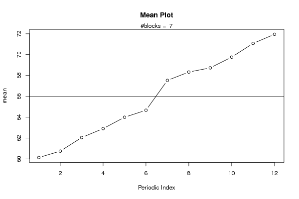
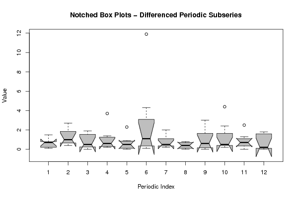
| Title produced by software | Mean Plot | ||||||||||||||||||||
| Date of computation | Sun, 20 May 2012 06:57:41 -0400 | ||||||||||||||||||||
| Cite this page as follows | Statistical Computations at FreeStatistics.org, Office for Research Development and Education, URL https://freestatistics.org/blog/index.php?v=date/2012/May/20/t1337511585ifee74cgh4wqsa6.htm/, Retrieved Tue, 30 Apr 2024 02:18:15 +0000 | ||||||||||||||||||||
| Statistical Computations at FreeStatistics.org, Office for Research Development and Education, URL https://freestatistics.org/blog/index.php?pk=166773, Retrieved Tue, 30 Apr 2024 02:18:15 +0000 | |||||||||||||||||||||
| QR Codes: | |||||||||||||||||||||
|
| |||||||||||||||||||||
| Original text written by user: | |||||||||||||||||||||
| IsPrivate? | No (this computation is public) | ||||||||||||||||||||
| User-defined keywords | KDG201162 | ||||||||||||||||||||
| Estimated Impact | 124 | ||||||||||||||||||||
Tree of Dependent Computations | |||||||||||||||||||||
| Family? (F = Feedback message, R = changed R code, M = changed R Module, P = changed Parameters, D = changed Data) | |||||||||||||||||||||
| - [Mean Plot] [] [2011-10-24 11:50:03] [c804c9d9debe6cbacd66d26bebf6dd2f] - R D [Mean Plot] [] [2012-05-20 10:57:41] [21ca38b5c207d9fbe3078e977c625188] [Current] | |||||||||||||||||||||
| Feedback Forum | |||||||||||||||||||||
Post a new message | |||||||||||||||||||||
Dataset | |||||||||||||||||||||
| Dataseries X: | |||||||||||||||||||||
31,1 31,8 32,5 34,4 35,5 35,5 36,6 37,1 37,9 38,1 39 41,5 41,8 41,9 44,6 46,1 46,4 47,2 47,7 49,2 49,3 49,3 49,5 50,1 51,9 52,6 53,2 53,5 53,7 53,7 53,9 54,1 54,8 55,4 55,9 56,8 58,4 59,3 60,3 60,5 60,8 61 61,1 61,3 61,4 61,5 63,9 63,9 64 64,1 64,5 64,5 65,9 66,8 68,7 69,2 69,6 70,2 70,6 70,7 70,7 71 72,1 73,7 77,4 79,7 91,6 93,6 94,3 97,3 101,7 103 103,1 104,6 107,2 107,7 108,3 108,8 113,1 113,8 113,8 116,5 116,9 117,6 | |||||||||||||||||||||
Tables (Output of Computation) | |||||||||||||||||||||
| |||||||||||||||||||||
Figures (Output of Computation) | |||||||||||||||||||||
Input Parameters & R Code | |||||||||||||||||||||
| Parameters (Session): | |||||||||||||||||||||
| par1 = 12 ; | |||||||||||||||||||||
| Parameters (R input): | |||||||||||||||||||||
| par1 = 12 ; | |||||||||||||||||||||
| R code (references can be found in the software module): | |||||||||||||||||||||
par1 <- as.numeric(par1) | |||||||||||||||||||||