Free Statistics
of Irreproducible Research!
Description of Statistical Computation | |||||||||||||||||||||
|---|---|---|---|---|---|---|---|---|---|---|---|---|---|---|---|---|---|---|---|---|---|
| Author's title | |||||||||||||||||||||
| Author | *Unverified author* | ||||||||||||||||||||
| R Software Module | rwasp_sdplot.wasp | ||||||||||||||||||||
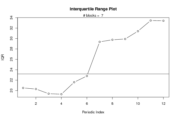
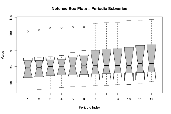
| Title produced by software | Standard Deviation Plot | ||||||||||||||||||||
| Date of computation | Mon, 21 May 2012 04:17:21 -0400 | ||||||||||||||||||||
| Cite this page as follows | Statistical Computations at FreeStatistics.org, Office for Research Development and Education, URL https://freestatistics.org/blog/index.php?v=date/2012/May/21/t13375884208j0658qnipdiokr.htm/, Retrieved Thu, 02 May 2024 13:57:05 +0000 | ||||||||||||||||||||
| Statistical Computations at FreeStatistics.org, Office for Research Development and Education, URL https://freestatistics.org/blog/index.php?pk=166883, Retrieved Thu, 02 May 2024 13:57:05 +0000 | |||||||||||||||||||||
| QR Codes: | |||||||||||||||||||||
|
| |||||||||||||||||||||
| Original text written by user: | |||||||||||||||||||||
| IsPrivate? | No (this computation is public) | ||||||||||||||||||||
| User-defined keywords | KDGP2W83 | ||||||||||||||||||||
| Estimated Impact | 112 | ||||||||||||||||||||
Tree of Dependent Computations | |||||||||||||||||||||
| Family? (F = Feedback message, R = changed R code, M = changed R Module, P = changed Parameters, D = changed Data) | |||||||||||||||||||||
| - [Bootstrap Plot - Central Tendency] [Bootstrap Plot va...] [2012-05-02 19:39:36] [562ee1d5a96d07a2dc4978b28f7ac089] - RMPD [Blocked Bootstrap Plot - Central Tendency] [Blocked Bootstrap...] [2012-05-02 19:52:56] [562ee1d5a96d07a2dc4978b28f7ac089] - RMPD [Standard Deviation Plot] [Standard Deviatio...] [2012-05-02 20:02:11] [562ee1d5a96d07a2dc4978b28f7ac089] - PD [Standard Deviation Plot] [] [2012-05-21 08:17:21] [21ca38b5c207d9fbe3078e977c625188] [Current] | |||||||||||||||||||||
| Feedback Forum | |||||||||||||||||||||
Post a new message | |||||||||||||||||||||
Dataset | |||||||||||||||||||||
| Dataseries X: | |||||||||||||||||||||
31.1 31.8 32.5 34.4 35.5 35.5 36.6 37.1 37.9 38.1 39 41.5 41.8 41.9 44.6 46.1 46.4 47.2 47.7 49.2 49.3 49.3 49.5 50.1 51.9 52.6 53.2 53.5 53.7 53.7 53.9 54.1 54.8 55.4 55.9 56.8 58.4 59.3 60.3 60.5 60.8 61 61.1 61.3 61.4 61.5 63.9 63.9 64 64.1 64.5 64.5 65.9 66.8 68.7 69.2 69.6 70.2 70.6 70.7 70.7 71 72.1 73.7 77.4 79.7 91.6 93.6 94.3 97.3 101.7 103 103.1 104.6 107.2 107.7 108.3 108.8 113.1 113.8 113.8 116.5 116.9 117.6 | |||||||||||||||||||||
Tables (Output of Computation) | |||||||||||||||||||||
| |||||||||||||||||||||
Figures (Output of Computation) | |||||||||||||||||||||
Input Parameters & R Code | |||||||||||||||||||||
| Parameters (Session): | |||||||||||||||||||||
| par1 = 12 ; | |||||||||||||||||||||
| Parameters (R input): | |||||||||||||||||||||
| par1 = 12 ; | |||||||||||||||||||||
| R code (references can be found in the software module): | |||||||||||||||||||||
par1 <- as.numeric(par1) | |||||||||||||||||||||