Free Statistics
of Irreproducible Research!
Description of Statistical Computation | |||||||||||||||||||||
|---|---|---|---|---|---|---|---|---|---|---|---|---|---|---|---|---|---|---|---|---|---|
| Author's title | |||||||||||||||||||||
| Author | *Unverified author* | ||||||||||||||||||||
| R Software Module | rwasp_meanplot.wasp | ||||||||||||||||||||
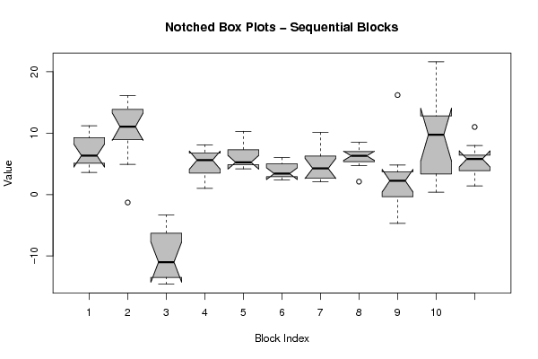
| Title produced by software | Mean Plot | ||||||||||||||||||||
| Date of computation | Mon, 28 May 2012 11:50:14 -0400 | ||||||||||||||||||||
| Cite this page as follows | Statistical Computations at FreeStatistics.org, Office for Research Development and Education, URL https://freestatistics.org/blog/index.php?v=date/2012/May/28/t1338220240yrhoq0rf45kzh1d.htm/, Retrieved Thu, 02 May 2024 06:47:31 +0000 | ||||||||||||||||||||
| Statistical Computations at FreeStatistics.org, Office for Research Development and Education, URL https://freestatistics.org/blog/index.php?pk=167824, Retrieved Thu, 02 May 2024 06:47:31 +0000 | |||||||||||||||||||||
| QR Codes: | |||||||||||||||||||||
|
| |||||||||||||||||||||
| Original text written by user: | |||||||||||||||||||||
| IsPrivate? | No (this computation is public) | ||||||||||||||||||||
| User-defined keywords | KDG201162 | ||||||||||||||||||||
| Estimated Impact | 112 | ||||||||||||||||||||
Tree of Dependent Computations | |||||||||||||||||||||
| Family? (F = Feedback message, R = changed R code, M = changed R Module, P = changed Parameters, D = changed Data) | |||||||||||||||||||||
| - [(Partial) Autocorrelation Function] [KDGP2W12] [2012-04-07 16:19:00] [6285f4e2f27456c551d88825e9bb3ea0] - RMP [Mean Plot] [KDG201162] [2012-05-28 15:50:14] [d77480184cff5133157c4adeb3391928] [Current] | |||||||||||||||||||||
| Feedback Forum | |||||||||||||||||||||
Post a new message | |||||||||||||||||||||
Dataset | |||||||||||||||||||||
| Dataseries X: | |||||||||||||||||||||
3,9 5,9 5,7 3,6 4,9 5,3 8,7 6,8 8,9 9,6 11,2 9,9 9,3 9,2 9,4 12,7 13,6 16,1 14,8 14,1 13,2 8,7 4,9 -1,3 -3,9 -6 -6,6 -8,7 -11,6 -14,6 -12,9 -13,8 -14,1 -13,2 -10,4 -3,3 1 3,1 4,5 1,9 3,9 7 5,6 8,1 6,1 8 6,5 5,6 4,8 5,1 7,8 10,3 8,6 6,8 4,9 5,4 5,5 4,7 4,2 5 5 6 2,9 3,6 5,1 2,9 4,7 3 5 2,6 3,2 2,4 3,2 2,6 2,4 2,1 2,7 4,4 4,3 4,2 5,5 8,8 10,1 7 5,7 5,2 5,5 7,3 5,9 7,1 6,9 6,7 4,7 6,7 8,5 2,1 -0,9 -4,7 4,8 2,6 1,7 -1,8 0,2 1,9 3,2 3,1 4,2 16,2 18,3 21,6 12,6 9,8 10,6 13 9,7 7,9 3,3 3,4 0,4 0,7 1,4 3,8 4 8 6 5,8 3,9 6,4 11 | |||||||||||||||||||||
Tables (Output of Computation) | |||||||||||||||||||||
| |||||||||||||||||||||
Figures (Output of Computation) | |||||||||||||||||||||
Input Parameters & R Code | |||||||||||||||||||||
| Parameters (Session): | |||||||||||||||||||||
| par1 = 12 ; | |||||||||||||||||||||
| Parameters (R input): | |||||||||||||||||||||
| par1 = 12 ; | |||||||||||||||||||||
| R code (references can be found in the software module): | |||||||||||||||||||||
par1 <- as.numeric(par1) | |||||||||||||||||||||