Free Statistics
of Irreproducible Research!
Description of Statistical Computation | |||||||||||||||||||||
|---|---|---|---|---|---|---|---|---|---|---|---|---|---|---|---|---|---|---|---|---|---|
| Author's title | |||||||||||||||||||||
| Author | *Unverified author* | ||||||||||||||||||||
| R Software Module | rwasp_meanplot.wasp | ||||||||||||||||||||
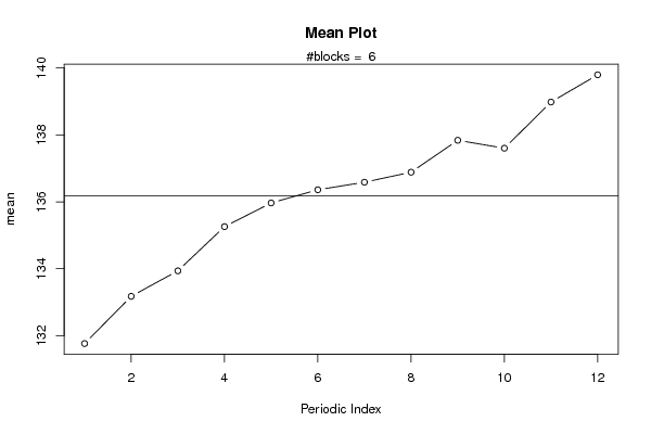
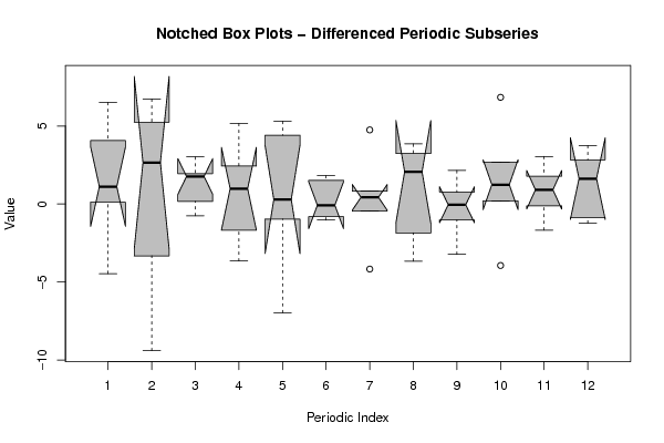
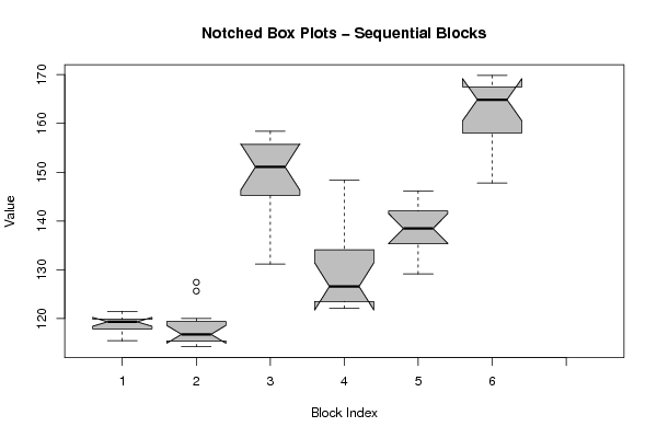
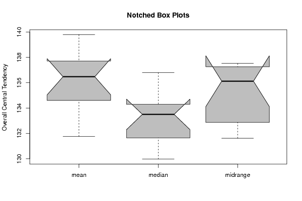
| Title produced by software | Mean Plot | ||||||||||||||||||||
| Date of computation | Mon, 28 May 2012 16:07:55 -0400 | ||||||||||||||||||||
| Cite this page as follows | Statistical Computations at FreeStatistics.org, Office for Research Development and Education, URL https://freestatistics.org/blog/index.php?v=date/2012/May/28/t13382357392u9bqvj1a1p6xso.htm/, Retrieved Wed, 01 May 2024 23:38:04 +0000 | ||||||||||||||||||||
| Statistical Computations at FreeStatistics.org, Office for Research Development and Education, URL https://freestatistics.org/blog/index.php?pk=167873, Retrieved Wed, 01 May 2024 23:38:04 +0000 | |||||||||||||||||||||
| QR Codes: | |||||||||||||||||||||
|
| |||||||||||||||||||||
| Original text written by user: | |||||||||||||||||||||
| IsPrivate? | No (this computation is public) | ||||||||||||||||||||
| User-defined keywords | KDG201162 | ||||||||||||||||||||
| Estimated Impact | 84 | ||||||||||||||||||||
Tree of Dependent Computations | |||||||||||||||||||||
| Family? (F = Feedback message, R = changed R code, M = changed R Module, P = changed Parameters, D = changed Data) | |||||||||||||||||||||
| - [Mean Plot] [Opgave 6 oef 2] [2012-05-28 20:07:55] [919141dca056cde38faaf6352f12d0de] [Current] | |||||||||||||||||||||
| Feedback Forum | |||||||||||||||||||||
Post a new message | |||||||||||||||||||||
Dataset | |||||||||||||||||||||
| Dataseries X: | |||||||||||||||||||||
115,43 115,55 117,14 119,09 119,55 119,8 121,32 121,48 119,63 118,61 118,82 119,93 118,7 119,99 116,67 116,84 115,17 114,21 114,77 115,59 116,64 118,79 125,63 127,42 131,17 137,68 144,41 146,09 151,26 156,56 158,38 154,21 158,06 154,83 150,89 149,22 148,34 143,88 134,48 133,73 130,08 123,11 122,08 126,83 123,17 123,82 125,6 126,32 129,15 130,09 133,81 136,83 138,34 138,67 137,86 138,56 141,65 142,42 143,12 146,17 147,8 151,87 157,12 158,97 161,4 165,81 165,1 164,64 167,88 167,14 169,83 169,71 | |||||||||||||||||||||
Tables (Output of Computation) | |||||||||||||||||||||
| |||||||||||||||||||||
Figures (Output of Computation) | |||||||||||||||||||||
Input Parameters & R Code | |||||||||||||||||||||
| Parameters (Session): | |||||||||||||||||||||
| par1 = 12 ; | |||||||||||||||||||||
| Parameters (R input): | |||||||||||||||||||||
| par1 = 12 ; | |||||||||||||||||||||
| R code (references can be found in the software module): | |||||||||||||||||||||
par1 <- as.numeric(par1) | |||||||||||||||||||||