Free Statistics
of Irreproducible Research!
Description of Statistical Computation | |||||||||||||||||||||
|---|---|---|---|---|---|---|---|---|---|---|---|---|---|---|---|---|---|---|---|---|---|
| Author's title | |||||||||||||||||||||
| Author | *Unverified author* | ||||||||||||||||||||
| R Software Module | rwasp_meanplot.wasp | ||||||||||||||||||||
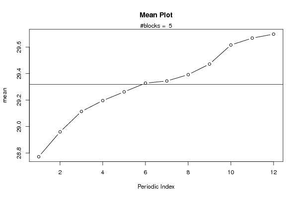
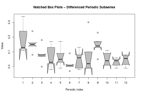
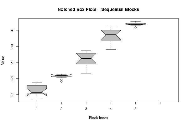
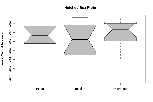
| Title produced by software | Mean Plot | ||||||||||||||||||||
| Date of computation | Tue, 29 May 2012 04:59:06 -0400 | ||||||||||||||||||||
| Cite this page as follows | Statistical Computations at FreeStatistics.org, Office for Research Development and Education, URL https://freestatistics.org/blog/index.php?v=date/2012/May/29/t1338282391ydsxcqx9wekxywg.htm/, Retrieved Mon, 29 Apr 2024 21:47:36 +0000 | ||||||||||||||||||||
| Statistical Computations at FreeStatistics.org, Office for Research Development and Education, URL https://freestatistics.org/blog/index.php?pk=167954, Retrieved Mon, 29 Apr 2024 21:47:36 +0000 | |||||||||||||||||||||
| QR Codes: | |||||||||||||||||||||
|
| |||||||||||||||||||||
| Original text written by user: | |||||||||||||||||||||
| IsPrivate? | No (this computation is public) | ||||||||||||||||||||
| User-defined keywords | KDG201162 | ||||||||||||||||||||
| Estimated Impact | 112 | ||||||||||||||||||||
Tree of Dependent Computations | |||||||||||||||||||||
| Family? (F = Feedback message, R = changed R code, M = changed R Module, P = changed Parameters, D = changed Data) | |||||||||||||||||||||
| - [Histogram] [Opgave 2 stap 2] [2012-05-29 06:48:13] [46972ec2bfa5b295f8450f947ab1f239] - RMPD [Mean Plot] [Opgave 6 oefening 2 ] [2012-05-29 08:59:06] [7d6606cca1b3596736d7d387043cb02b] [Current] | |||||||||||||||||||||
| Feedback Forum | |||||||||||||||||||||
Post a new message | |||||||||||||||||||||
Dataset | |||||||||||||||||||||
| Dataseries X: | |||||||||||||||||||||
26,73 26,85 27,01 27,09 27,11 27,16 27,13 27,19 27,49 27,63 27,72 27,77 27,81 27,92 28,07 28,14 28,17 28,2 28,21 28,2 28,19 28,24 28,25 28,26 28,33 28,67 28,81 28,99 29,16 29,25 29,25 29,38 29,48 29,65 29,69 29,73 29,81 30,05 30,29 30,37 30,5 30,67 30,76 30,84 30,86 31,09 31,2 31,19 31,18 31,31 31,39 31,39 31,37 31,36 31,37 31,35 31,34 31,47 31,48 31,54 | |||||||||||||||||||||
Tables (Output of Computation) | |||||||||||||||||||||
| |||||||||||||||||||||
Figures (Output of Computation) | |||||||||||||||||||||
Input Parameters & R Code | |||||||||||||||||||||
| Parameters (Session): | |||||||||||||||||||||
| Parameters (R input): | |||||||||||||||||||||
| par1 = 12 ; | |||||||||||||||||||||
| R code (references can be found in the software module): | |||||||||||||||||||||
par1 <- as.numeric(par1) | |||||||||||||||||||||