Free Statistics
of Irreproducible Research!
Description of Statistical Computation | |||||||||||||||||||||||||||||||||||||||||||||||||||||
|---|---|---|---|---|---|---|---|---|---|---|---|---|---|---|---|---|---|---|---|---|---|---|---|---|---|---|---|---|---|---|---|---|---|---|---|---|---|---|---|---|---|---|---|---|---|---|---|---|---|---|---|---|---|
| Author's title | |||||||||||||||||||||||||||||||||||||||||||||||||||||
| Author | *The author of this computation has been verified* | ||||||||||||||||||||||||||||||||||||||||||||||||||||
| R Software Module | rwasp_edauni.wasp | ||||||||||||||||||||||||||||||||||||||||||||||||||||
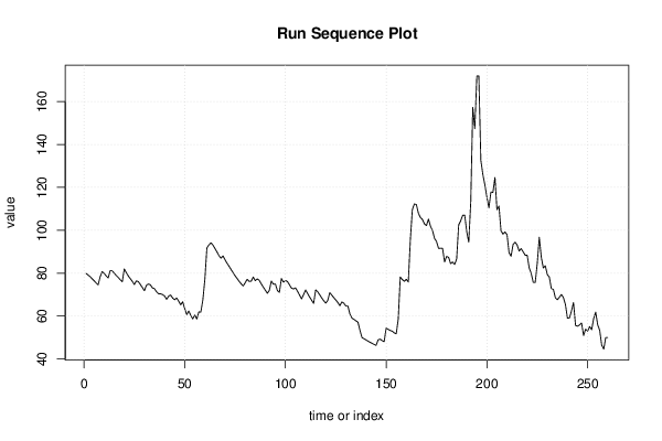
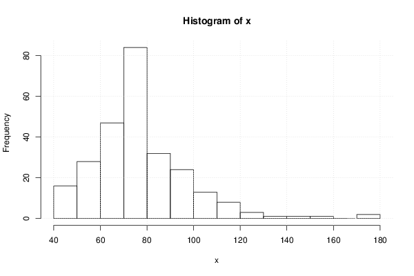
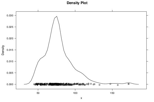
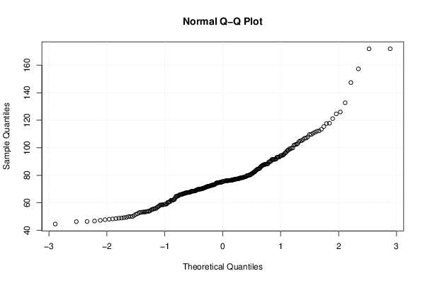
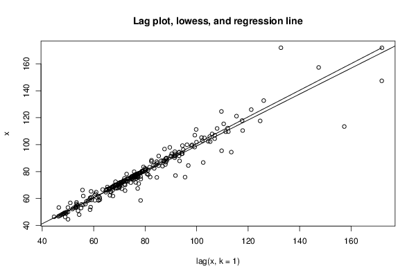
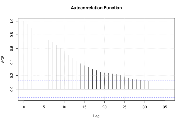
| Title produced by software | Univariate Explorative Data Analysis | ||||||||||||||||||||||||||||||||||||||||||||||||||||
| Date of computation | Tue, 13 Nov 2012 18:41:06 -0500 | ||||||||||||||||||||||||||||||||||||||||||||||||||||
| Cite this page as follows | Statistical Computations at FreeStatistics.org, Office for Research Development and Education, URL https://freestatistics.org/blog/index.php?v=date/2012/Nov/13/t1352850082ss075wnihwzg2ne.htm/, Retrieved Sun, 28 Apr 2024 14:30:41 +0000 | ||||||||||||||||||||||||||||||||||||||||||||||||||||
| Statistical Computations at FreeStatistics.org, Office for Research Development and Education, URL https://freestatistics.org/blog/index.php?pk=189215, Retrieved Sun, 28 Apr 2024 14:30:41 +0000 | |||||||||||||||||||||||||||||||||||||||||||||||||||||
| QR Codes: | |||||||||||||||||||||||||||||||||||||||||||||||||||||
|
| |||||||||||||||||||||||||||||||||||||||||||||||||||||
| Original text written by user: | |||||||||||||||||||||||||||||||||||||||||||||||||||||
| IsPrivate? | No (this computation is public) | ||||||||||||||||||||||||||||||||||||||||||||||||||||
| User-defined keywords | |||||||||||||||||||||||||||||||||||||||||||||||||||||
| Estimated Impact | 61 | ||||||||||||||||||||||||||||||||||||||||||||||||||||
Tree of Dependent Computations | |||||||||||||||||||||||||||||||||||||||||||||||||||||
| Family? (F = Feedback message, R = changed R code, M = changed R Module, P = changed Parameters, D = changed Data) | |||||||||||||||||||||||||||||||||||||||||||||||||||||
| - [Bivariate Data Series] [Bivariate dataset] [2008-01-05 23:51:08] [74be16979710d4c4e7c6647856088456] F RMPD [Univariate Explorative Data Analysis] [Colombia Coffee] [2008-01-07 14:21:11] [74be16979710d4c4e7c6647856088456] - RMPD [Univariate Explorative Data Analysis] [winsorize] [2012-11-13 23:41:06] [2f047a68beb18e789d06219c4ebd4599] [Current] | |||||||||||||||||||||||||||||||||||||||||||||||||||||
| Feedback Forum | |||||||||||||||||||||||||||||||||||||||||||||||||||||
Post a new message | |||||||||||||||||||||||||||||||||||||||||||||||||||||
Dataset | |||||||||||||||||||||||||||||||||||||||||||||||||||||
| Dataseries X: | |||||||||||||||||||||||||||||||||||||||||||||||||||||
79,88 79,16 78,38 77,42 76,47 75,46 74,48 78,27 80,7 79,91 78,75 77,78 81,14 81,08 80,03 78,91 78,01 76,9 75,97 81,93 80,27 78,67 77,42 76,16 74,7 76,39 76,04 74,65 73,29 71,79 74,39 74,91 74,54 73,08 72,75 71,32 70,38 70,35 70,01 69,36 67,77 69,26 69,8 68,38 67,62 68,39 66,95 65,21 66,64 63,45 60,66 62,34 60,32 58,64 60,46 58,59 61,87 61,85 67,44 77,06 91,74 93,15 94,15 93,11 91,51 89,96 88,16 86,98 88,03 86,24 84,65 83,23 81,7 80,25 78,8 77,51 76,2 75,04 74 75,49 77,14 76,15 76,27 78,19 76,49 77,31 76,65 74,99 73,51 72,07 70,59 71,96 76,29 74,86 74,93 71,9 71,01 77,47 75,78 76,6 76,07 74,57 73,02 72,65 73,16 71,53 69,78 67,98 69,96 72,16 70,47 68,86 67,37 65,87 72,16 71,34 69,93 68,44 67,16 66,01 67,25 70,91 69,75 68,59 67,48 66,31 64,81 66,58 65,97 64,7 64,7 60,94 59,08 58,42 57,77 57,11 53,31 49,96 49,4 48,84 48,3 47,74 47,24 46,76 46,29 48,9 49,23 48,53 48,03 54,34 53,79 53,24 52,96 52,17 51,7 58,55 78,2 77,03 76,19 77,15 75,87 95,47 109,67 112,28 112,01 107,93 105,96 105,06 102,98 102,2 105,23 101,85 99,89 96,23 94,76 91,51 91,63 91,54 85,23 87,83 87,38 84,44 85,19 84,03 86,73 102,52 104,45 106,98 107,02 99,26 94,45 113,44 157,33 147,38 171,89 171,95 132,71 126,02 121,18 115,45 110,48 117,85 117,63 124,65 109,59 111,27 99,78 98,21 99,2 97,97 89,55 87,91 93,34 94,42 93,2 90,29 91,46 89,98 88,35 88,41 82,44 79,89 75,69 75,66 84,5 96,73 87,48 82,39 83,48 79,31 78,16 72,77 72,45 68,46 67,62 68,76 70,07 68,55 65,3 58,96 59,17 62,37 66,28 55,62 55,23 55,85 56,75 50,89 53,88 52,95 55,08 53,61 58,78 61,85 55,91 53,32 46,41 44,57 50 50 | |||||||||||||||||||||||||||||||||||||||||||||||||||||
Tables (Output of Computation) | |||||||||||||||||||||||||||||||||||||||||||||||||||||
| |||||||||||||||||||||||||||||||||||||||||||||||||||||
Figures (Output of Computation) | |||||||||||||||||||||||||||||||||||||||||||||||||||||
Input Parameters & R Code | |||||||||||||||||||||||||||||||||||||||||||||||||||||
| Parameters (Session): | |||||||||||||||||||||||||||||||||||||||||||||||||||||
| par1 = 0 ; par2 = 36 ; | |||||||||||||||||||||||||||||||||||||||||||||||||||||
| Parameters (R input): | |||||||||||||||||||||||||||||||||||||||||||||||||||||
| par1 = 0 ; par2 = 36 ; | |||||||||||||||||||||||||||||||||||||||||||||||||||||
| R code (references can be found in the software module): | |||||||||||||||||||||||||||||||||||||||||||||||||||||
par1 <- as.numeric(par1) | |||||||||||||||||||||||||||||||||||||||||||||||||||||