Repository of Reproducible Computations

Free Statistics

of Irreproducible Research!

Author's title

Author

*The author of this computation has been verified*

R Software Module

rwasp_CARE Data Boxplot.wasp

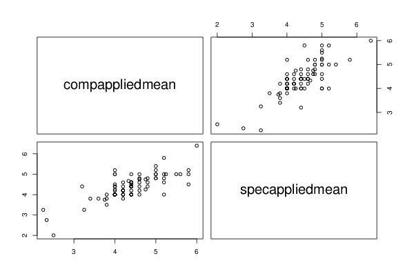
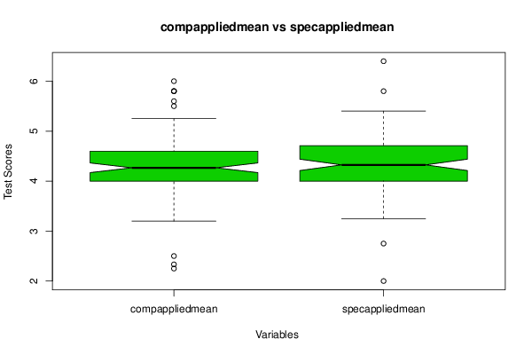
Title produced by software

CARE Data - Boxplots and Scatterplot Matrix

Date of computation

Mon, 19 Nov 2012 14:22:49 -0500

Cite this page as follows

Statistical Computations at FreeStatistics.org, Office for Research Development and Education, URL https://freestatistics.org/blog/index.php?v=date/2012/Nov/19/t1353352991in06leyso9qrr8w.htm/, Retrieved Sat, 27 Apr 2024 23:56:15 +0000

Statistical Computations at FreeStatistics.org, Office for Research Development and Education, URL https://freestatistics.org/blog/index.php?pk=190746, Retrieved Sat, 27 Apr 2024 23:56:15 +0000

QR Codes:

Paste this QR Code to cite your computation.

Original text written by user:

IsPrivate?

No (this computation is public)

User-defined keywords

Estimated Impact

Family? (F = Feedback message, R = changed R code, M = changed R Module, P = changed Parameters, D = changed Data)

-     [Correlation] [Shapiro Wilkes co...] [2012-11-19 17:28:33] [7cd3c6995ee3ebd1d961fab932753011]
- R P   [Correlation] [Kendalls compmemo...] [2012-11-19 17:33:59] [7cd3c6995ee3ebd1d961fab932753011]
-   P     [Correlation] [Spearmen's rho co...] [2012-11-19 17:44:52] [7cd3c6995ee3ebd1d961fab932753011]
-   PD      [Correlation] [Shapiro Wilkes co...] [2012-11-19 17:58:42] [7cd3c6995ee3ebd1d961fab932753011]
-    D        [Correlation] [Shapiro Wilkes co...] [2012-11-19 18:18:55] [7cd3c6995ee3ebd1d961fab932753011]
-               [Correlation] [Spearmens rho com...] [2012-11-19 18:25:03] [7cd3c6995ee3ebd1d961fab932753011]
-    D            [Correlation] [Shapiro Wilkes co...] [2012-11-19 18:48:00] [7cd3c6995ee3ebd1d961fab932753011]
-                   [Correlation] [Kendalls Tau comp...] [2012-11-19 18:52:29] [7cd3c6995ee3ebd1d961fab932753011]
-    D                [Correlation] [Shapiro Wilkes co...] [2012-11-19 18:59:49] [7cd3c6995ee3ebd1d961fab932753011]
-    D                  [Correlation] [Shapiro Wilkes co...] [2012-11-19 19:10:53] [7cd3c6995ee3ebd1d961fab932753011]
-                         [Correlation] [] [2012-11-19 19:13:15] [7cd3c6995ee3ebd1d961fab932753011]
-    D                      [Correlation] [] [2012-11-19 19:18:26] [7cd3c6995ee3ebd1d961fab932753011]
- RM D                          [CARE Data - Boxplots and Scatterplot Matrix] [] [2012-11-19 19:22:49] [bf8101b62fb6ce8682f2968a78253f3c] [Current]

Feedback Forum

Post a new message

Dataseries X:

Download CSV

Histogram

Boxplots

4.4	4.6
4.2	4
5.2	4.8
5.2	4
4.4	5
5.5	5
4	4
4	4
4	4.4
3.8	4
4	4
5.25	5
3.6	3.8
4.4	4.6
4	4
4.4	4.6
4.333333333	4.666666667
4.6	4
4	4
4.4	4.4
5	4.8
5.2	5.8
5.2	4.6
4.6	4.75
4.6	5
2.333333333	2.75
4	4
3.8	3.8
4	4.4
4.6	4.8
4.75	4.25
4.4	4.4
4	4
4	4.5
5.2	5
3.8	3.5
2.5	2
3.2	4.4
4.2	4.4
4	4.25
3.25	3.25
4.2	4.2
4.75	4.75
4.4	4.4
4	4
4.2	4.2
4	5
4.2	4.6
4.4	4.4
4	4
4.6	4.4
4.4	4.5
4	5.2
4.8	4.4
2.25	3.25
4.8	4.6
3.75	3.75
5.6	5
4.2	3.8
4.2	4
5	5.4
5.8	5
5	5
4	4.2
4.4	4.4
4.4	4
4.4	4.6
4.4	4.2
5.8	5.2
6	6.4
4	4
4	4
5	5
4	4
4.2	4.2
4.4	4
4	4
4	4
4	4
4.2	4
4.6	4.2
4.4	4
4.4	4
4	4
5	5.2
4.2	4.2
5	4.8
4	4
4.8	4.8
4	5
4.6	4.6
4	4
4.4	4.4
4	4
3.4	3.8
5.8	4.5

Summary of computational transaction
Raw Input	view raw input (R code)
Raw Output	view raw output of R engine
Computing time	2 seconds
R Server	'Sir Ronald Aylmer Fisher' @ fisher.wessa.net

\begin{tabular}{lllllllll}
\hline
Summary of computational transaction \tabularnewline
Raw Input & view raw input (R code)  \tabularnewline
Raw Output & view raw output of R engine  \tabularnewline
Computing time & 2 seconds \tabularnewline
R Server & 'Sir Ronald Aylmer Fisher' @ fisher.wessa.net \tabularnewline
\hline
\end{tabular}
%Source: https://freestatistics.org/blog/index.php?pk=190746&T=0

[TABLE]
[ROW][C]Summary of computational transaction[/C][/ROW]
[ROW][C]Raw Input[/C][C]view raw input (R code) [/C][/ROW]
[ROW][C]Raw Output[/C][C]view raw output of R engine [/C][/ROW]
[ROW][C]Computing time[/C][C]2 seconds[/C][/ROW]
[ROW][C]R Server[/C][C]'Sir Ronald Aylmer Fisher' @ fisher.wessa.net[/C][/ROW]
[/TABLE]
Source: https://freestatistics.org/blog/index.php?pk=190746&T=0

Globally Unique Identifier (entire table): ba.freestatistics.org/blog/index.php?pk=190746&T=0

As an alternative you can also use a QR Code:

The GUIDs for individual cells are displayed in the table below:

Summary of computational transaction
Raw Input	view raw input (R code)
Raw Output	view raw output of R engine
Computing time	2 seconds
R Server	'Sir Ronald Aylmer Fisher' @ fisher.wessa.net

Boxplot statistics
Variable	lower whisker	lower hinge	median	upper hinge	upper whisker
compappliedmean	3.2	4	4.267	4.6	5.25
specappliedmean	3.25	4	4.325	4.708	5.4

\begin{tabular}{lllllllll}
\hline
Boxplot statistics \tabularnewline
Variable & lower whisker & lower hinge & median & upper hinge & upper whisker \tabularnewline
compappliedmean & 3.2 & 4 & 4.267 & 4.6 & 5.25 \tabularnewline
specappliedmean & 3.25 & 4 & 4.325 & 4.708 & 5.4 \tabularnewline
\hline
\end{tabular}
%Source: https://freestatistics.org/blog/index.php?pk=190746&T=1

[TABLE]
[ROW][C]Boxplot statistics[/C][/ROW]
[ROW][C]Variable[/C][C]lower whisker[/C][C]lower hinge[/C][C]median[/C][C]upper hinge[/C][C]upper whisker[/C][/ROW]
[ROW][C]compappliedmean[/C][C]3.2[/C][C]4[/C][C]4.267[/C][C]4.6[/C][C]5.25[/C][/ROW]
[ROW][C]specappliedmean[/C][C]3.25[/C][C]4[/C][C]4.325[/C][C]4.708[/C][C]5.4[/C][/ROW]
[/TABLE]
Source: https://freestatistics.org/blog/index.php?pk=190746&T=1

Globally Unique Identifier (entire table): ba.freestatistics.org/blog/index.php?pk=190746&T=1

As an alternative you can also use a QR Code:

The GUIDs for individual cells are displayed in the table below:

Boxplot statistics
Variable	lower whisker	lower hinge	median	upper hinge	upper whisker
compappliedmean	3.2	4	4.267	4.6	5.25
specappliedmean	3.25	4	4.325	4.708	5.4

Boxplot Notches
Variable	lower bound	median	upper bound
compappliedmean	4.17	4.267	4.363
specappliedmean	4.211	4.325	4.439

\begin{tabular}{lllllllll}
\hline
Boxplot Notches \tabularnewline
Variable & lower bound & median & upper bound \tabularnewline
compappliedmean & 4.17 & 4.267 & 4.363 \tabularnewline
specappliedmean & 4.211 & 4.325 & 4.439 \tabularnewline
\hline
\end{tabular}
%Source: https://freestatistics.org/blog/index.php?pk=190746&T=2

[TABLE]
[ROW][C]Boxplot Notches[/C][/ROW]
[ROW][C]Variable[/C][C]lower bound[/C][C]median[/C][C]upper bound[/C][/ROW]
[ROW][C]compappliedmean[/C][C]4.17[/C][C]4.267[/C][C]4.363[/C][/ROW]
[ROW][C]specappliedmean[/C][C]4.211[/C][C]4.325[/C][C]4.439[/C][/ROW]
[/TABLE]
Source: https://freestatistics.org/blog/index.php?pk=190746&T=2

Globally Unique Identifier (entire table): ba.freestatistics.org/blog/index.php?pk=190746&T=2

As an alternative you can also use a QR Code:

The GUIDs for individual cells are displayed in the table below:

Boxplot Notches
Variable	lower bound	median	upper bound
compappliedmean	4.17	4.267	4.363
specappliedmean	4.211	4.325	4.439

Boxplot Means
Variable	trimmed mean	unbiased SD
compappliedmean	4.34	0.6567
specappliedmean	4.344	0.5874

\begin{tabular}{lllllllll}
\hline
Boxplot Means \tabularnewline
Variable & trimmed mean & unbiased SD \tabularnewline
compappliedmean & 4.34 & 0.6567 \tabularnewline
specappliedmean & 4.344 & 0.5874 \tabularnewline
\hline
\end{tabular}
%Source: https://freestatistics.org/blog/index.php?pk=190746&T=3

[TABLE]
[ROW][C]Boxplot Means[/C][/ROW]
[ROW][C]Variable[/C][C]trimmed mean[/C][C]unbiased SD[/C][/ROW]
[ROW][C]compappliedmean[/C][C]4.34[/C][C]0.6567[/C][/ROW]
[ROW][C]specappliedmean[/C][C]4.344[/C][C]0.5874[/C][/ROW]
[/TABLE]
Source: https://freestatistics.org/blog/index.php?pk=190746&T=3

Globally Unique Identifier (entire table): ba.freestatistics.org/blog/index.php?pk=190746&T=3

As an alternative you can also use a QR Code:

The GUIDs for individual cells are displayed in the table below:

Boxplot Means
Variable	trimmed mean	unbiased SD
compappliedmean	4.34	0.6567
specappliedmean	4.344	0.5874

Figure 1

PNG link

Postscript link

PDF link

Figure 2

PNG link

Postscript link

PDF link

Parameters (Session):

par1 = kendall ; par2 = two.sided ;

Parameters (R input):

par1 = 3 ; par2 = TRUE ; par3 = 0 ;

R code (references can be found in the software module):

par1 <- as.numeric(par1) #colour
par2<- as.logical(par2) # Notches ?
par3<-as.numeric(par3) # % trim
if(par3>45){par3<-45;warning('trim limited to 45%')}
if(par3<0){par3<-0;warning('negative trim makes no sense. Trim is zero.')}
lotrm<-as.integer(length(y[1,])*par3/100)+1
hitrm<-as.integer(length(y[1,])*(100-par3)/100)
y1<-array(dim=c(dim(y)[1], hitrm-lotrm+1), dimnames=list(dimnames(y)[[1]], 1:(hitrm-lotrm+1) ))
for(i in 1:dim(y)[1]){
tmp<-order(y[i,])
y1[i,]<- y[i, tmp[lotrm:hitrm] ]
}
bitmap(file='test2.png')
pairs(t(y))
dev.off()
y<-y1
z <- as.data.frame(t(y))
bitmap(file='test1.png')
(r<-boxplot(z ,xlab=xlab,ylab=ylab,main=main,notch=par2,col=par1))
dev.off()
load(file='createtable')
a<-table.start()
a<-table.row.start(a)
a<-table.element(a,hyperlink('overview.htm','Boxplot statistics','Boxplot overview'),6,TRUE)
a<-table.row.end(a)
a<-table.row.start(a)
a<-table.element(a,'Variable',1,TRUE)
a<-table.element(a,hyperlink('lower_whisker.htm','lower whisker','definition of lower whisker'),1,TRUE)
a<-table.element(a,hyperlink('lower_hinge.htm','lower hinge','definition of lower hinge'),1,TRUE)
a<-table.element(a,hyperlink('central_tendency.htm','median','definitions about measures of central tendency'),1,TRUE)
a<-table.element(a,hyperlink('upper_hinge.htm','upper hinge','definition of upper hinge'),1,TRUE)
a<-table.element(a,hyperlink('upper_whisker.htm','upper whisker','definition of upper whisker'),1,TRUE)
a<-table.row.end(a)
for (i in 1:length(y[,1]))
{
a<-table.row.start(a)
a<-table.element(a,dimnames(t(x))[[2]][i],1,TRUE)
for (j in 1:5)
{
a<-table.element(a,signif(r$stats[j,i], digits=4))
}
a<-table.row.end(a)
}
a<-table.end(a)
table.save(a,file='mytable.tab')
if (par2){
a<-table.start()
a<-table.row.start(a)
a<-table.element(a,'Boxplot Notches',4,TRUE)
a<-table.row.end(a)
a<-table.row.start(a)
a<-table.element(a,'Variable',1,TRUE)
a<-table.element(a,'lower bound',1,TRUE)
a<-table.element(a,'median',1,TRUE)
a<-table.element(a,'upper bound',1,TRUE)
a<-table.row.end(a)
for (i in 1:length(y[,1]))
{
a<-table.row.start(a)
a<-table.element(a,dimnames(t(x))[[2]][i],1,TRUE)
a<-table.element(a,signif(r$conf[1,i], digits=4))
a<-table.element(a, signif(r$stats[3,i], digits=4))
a<-table.element(a,signif(r$conf[2,i], digits=4))
a<-table.row.end(a)
}
a<-table.end(a)
table.save(a,file='mytable1.tab')
}
a<-table.start()
a<-table.row.start(a)
a<-table.element(a,'Boxplot Means',4,TRUE)
a<-table.row.end(a)
a<-table.row.start(a)
a<-table.element(a,'Variable',1,TRUE)
a<-table.element(a,hyperlink('trimmed_mean.htm','trimmed mean','definition of trimmed mean'),1,TRUE)
a<-table.element(a,hyperlink('unbiased1.htm','unbiased SD','definition of unbiased SD'),1,TRUE)
a<-table.row.end(a)
for (i in 1:length(y[,1]))
{
a<-table.row.start(a)
a<-table.element(a,dimnames(t(x))[[2]][i],1,TRUE)
a<-table.element(a,signif(mean(z[i], trim=par3/100, na.rm=TRUE), digits=4))
a<-table.element(a,signif(sd(z[i], na.rm=TRUE), digits=4))
a<-table.row.end(a)
}
a<-table.end(a)
table.save(a,file='mytable2.tab')

Free Statistics

Description of Statistical Computation

Tree of Dependent Computations

Dataset

Tables (Output of Computation)

Figures (Output of Computation)

Input Parameters & R Code