Free Statistics
of Irreproducible Research!
Description of Statistical Computation | |||||||||||||||||||||||||||||||||||||||||||||||||||||
|---|---|---|---|---|---|---|---|---|---|---|---|---|---|---|---|---|---|---|---|---|---|---|---|---|---|---|---|---|---|---|---|---|---|---|---|---|---|---|---|---|---|---|---|---|---|---|---|---|---|---|---|---|---|
| Author's title | |||||||||||||||||||||||||||||||||||||||||||||||||||||
| Author | *The author of this computation has been verified* | ||||||||||||||||||||||||||||||||||||||||||||||||||||
| R Software Module | rwasp_edauni.wasp | ||||||||||||||||||||||||||||||||||||||||||||||||||||
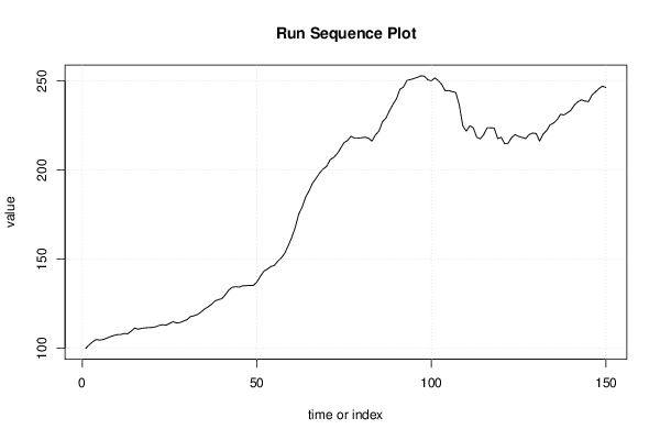
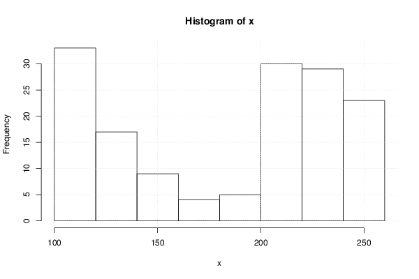
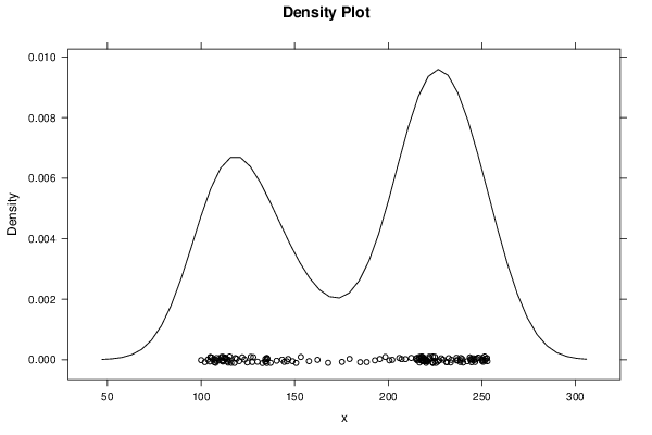
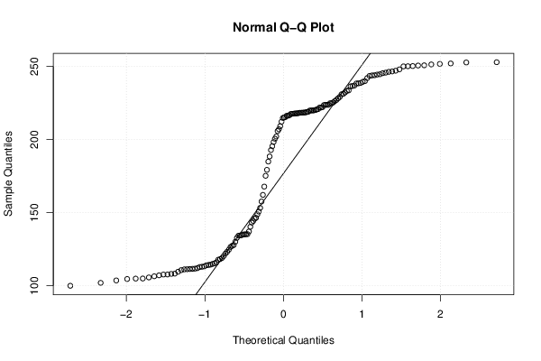
| Title produced by software | Univariate Explorative Data Analysis | ||||||||||||||||||||||||||||||||||||||||||||||||||||
| Date of computation | Mon, 19 Nov 2012 18:02:38 -0500 | ||||||||||||||||||||||||||||||||||||||||||||||||||||
| Cite this page as follows | Statistical Computations at FreeStatistics.org, Office for Research Development and Education, URL https://freestatistics.org/blog/index.php?v=date/2012/Nov/19/t1353366252i7aqbqt2zbtn7vx.htm/, Retrieved Sun, 28 Apr 2024 02:08:57 +0000 | ||||||||||||||||||||||||||||||||||||||||||||||||||||
| Statistical Computations at FreeStatistics.org, Office for Research Development and Education, URL https://freestatistics.org/blog/index.php?pk=190851, Retrieved Sun, 28 Apr 2024 02:08:57 +0000 | |||||||||||||||||||||||||||||||||||||||||||||||||||||
| QR Codes: | |||||||||||||||||||||||||||||||||||||||||||||||||||||
|
| |||||||||||||||||||||||||||||||||||||||||||||||||||||
| Original text written by user: | |||||||||||||||||||||||||||||||||||||||||||||||||||||
| IsPrivate? | No (this computation is public) | ||||||||||||||||||||||||||||||||||||||||||||||||||||
| User-defined keywords | |||||||||||||||||||||||||||||||||||||||||||||||||||||
| Estimated Impact | 56 | ||||||||||||||||||||||||||||||||||||||||||||||||||||
Tree of Dependent Computations | |||||||||||||||||||||||||||||||||||||||||||||||||||||
| Family? (F = Feedback message, R = changed R code, M = changed R Module, P = changed Parameters, D = changed Data) | |||||||||||||||||||||||||||||||||||||||||||||||||||||
| - [Univariate Explorative Data Analysis] [time effect in su...] [2010-11-17 08:55:33] [b98453cac15ba1066b407e146608df68] - R D [Univariate Explorative Data Analysis] [WS7.2] [2012-11-19 23:02:38] [6144fd9dab7e8876ce9100c6a2ac91c2] [Current] | |||||||||||||||||||||||||||||||||||||||||||||||||||||
| Feedback Forum | |||||||||||||||||||||||||||||||||||||||||||||||||||||
Post a new message | |||||||||||||||||||||||||||||||||||||||||||||||||||||
Dataset | |||||||||||||||||||||||||||||||||||||||||||||||||||||
| Dataseries X: | |||||||||||||||||||||||||||||||||||||||||||||||||||||
100 102 103,65 104,974 104,641 104,902 105,695 106,489 107,146 107,695 107,711 108,313 108,124 109,615 111,34 110,717 111,217 111,452 111,611 111,717 112,062 112,842 113,241 113,015 113,998 114,936 114,245 114,437 115,286 116,071 117,807 118,255 118,969 120,333 121,998 123,239 124,666 126,54 127,336 127,871 130,115 132,773 134,265 134,596 134,38 135,121 135,136 135,336 135,284 137,144 140,349 143,264 144,381 145,881 146,497 148,857 150,78 153,293 157,641 162,182 167,86 175,245 179,32 184,979 188,482 192,86 195,475 198,4 200,598 202,121 205,875 207,085 209,204 212,246 215,466 216,693 219,019 217,924 217,978 218,186 218,54 217,886 216,347 219,825 221,956 227,184 229,247 233,33 236,987 240,027 245,433 246,641 250,328 250,849 251,435 252,091 252,946 252,773 250,677 250,105 251,788 250,212 248,073 244,468 244,727 244,034 243,588 236,447 224,906 221,934 224,903 223,798 218,529 217,521 219,971 223,841 223,764 223,664 217,678 218,478 214,815 215,143 218,381 219,962 218,933 218,36 217,72 219,934 220,842 220,584 216,346 220,221 222,182 225,455 226,42 228,287 231,349 231,015 232,241 233,688 236,667 238,439 239,488 238,741 238,5 242,116 243,923 245,813 247,143 246,381 | |||||||||||||||||||||||||||||||||||||||||||||||||||||
Tables (Output of Computation) | |||||||||||||||||||||||||||||||||||||||||||||||||||||
| |||||||||||||||||||||||||||||||||||||||||||||||||||||
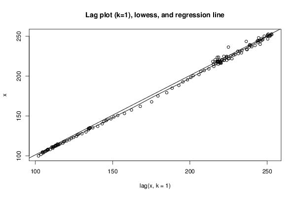
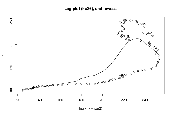
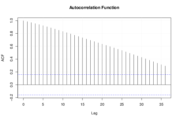
Figures (Output of Computation) | |||||||||||||||||||||||||||||||||||||||||||||||||||||
Input Parameters & R Code | |||||||||||||||||||||||||||||||||||||||||||||||||||||
| Parameters (Session): | |||||||||||||||||||||||||||||||||||||||||||||||||||||
| par1 = 0 ; par2 = 36 ; | |||||||||||||||||||||||||||||||||||||||||||||||||||||
| Parameters (R input): | |||||||||||||||||||||||||||||||||||||||||||||||||||||
| par1 = 0 ; par2 = 36 ; | |||||||||||||||||||||||||||||||||||||||||||||||||||||
| R code (references can be found in the software module): | |||||||||||||||||||||||||||||||||||||||||||||||||||||
par1 <- as.numeric(par1) | |||||||||||||||||||||||||||||||||||||||||||||||||||||