Free Statistics
of Irreproducible Research!
Description of Statistical Computation | |||||||||||||||||||||||||||||||||||||||||||||||||||||||||||||
|---|---|---|---|---|---|---|---|---|---|---|---|---|---|---|---|---|---|---|---|---|---|---|---|---|---|---|---|---|---|---|---|---|---|---|---|---|---|---|---|---|---|---|---|---|---|---|---|---|---|---|---|---|---|---|---|---|---|---|---|---|---|
| Author's title | |||||||||||||||||||||||||||||||||||||||||||||||||||||||||||||
| Author | *The author of this computation has been verified* | ||||||||||||||||||||||||||||||||||||||||||||||||||||||||||||
| R Software Module | rwasp_linear_regression.wasp | ||||||||||||||||||||||||||||||||||||||||||||||||||||||||||||
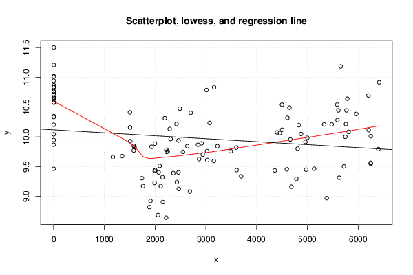
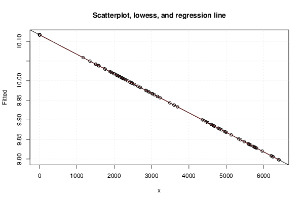
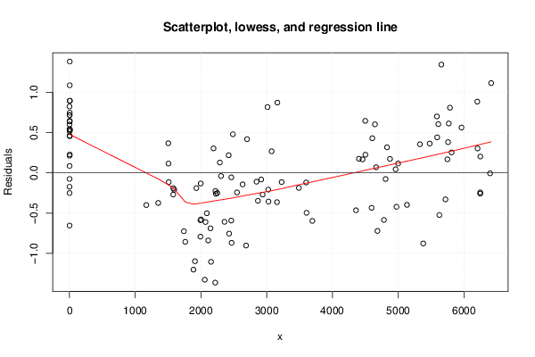
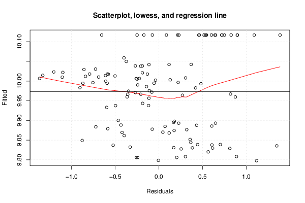
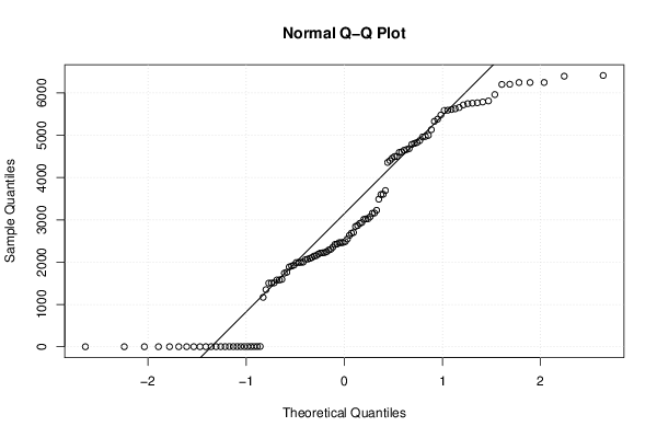
| Title produced by software | Linear Regression Graphical Model Validation | ||||||||||||||||||||||||||||||||||||||||||||||||||||||||||||
| Date of computation | Sat, 24 Nov 2012 19:32:20 -0500 | ||||||||||||||||||||||||||||||||||||||||||||||||||||||||||||
| Cite this page as follows | Statistical Computations at FreeStatistics.org, Office for Research Development and Education, URL https://freestatistics.org/blog/index.php?v=date/2012/Nov/24/t1353803628b4rtux1d4xa2tqh.htm/, Retrieved Sun, 28 Apr 2024 19:57:20 +0000 | ||||||||||||||||||||||||||||||||||||||||||||||||||||||||||||
| Statistical Computations at FreeStatistics.org, Office for Research Development and Education, URL https://freestatistics.org/blog/index.php?pk=192545, Retrieved Sun, 28 Apr 2024 19:57:20 +0000 | |||||||||||||||||||||||||||||||||||||||||||||||||||||||||||||
| QR Codes: | |||||||||||||||||||||||||||||||||||||||||||||||||||||||||||||
|
| |||||||||||||||||||||||||||||||||||||||||||||||||||||||||||||
| Original text written by user: | |||||||||||||||||||||||||||||||||||||||||||||||||||||||||||||
| IsPrivate? | No (this computation is public) | ||||||||||||||||||||||||||||||||||||||||||||||||||||||||||||
| User-defined keywords | |||||||||||||||||||||||||||||||||||||||||||||||||||||||||||||
| Estimated Impact | 123 | ||||||||||||||||||||||||||||||||||||||||||||||||||||||||||||
Tree of Dependent Computations | |||||||||||||||||||||||||||||||||||||||||||||||||||||||||||||
| Family? (F = Feedback message, R = changed R code, M = changed R Module, P = changed Parameters, D = changed Data) | |||||||||||||||||||||||||||||||||||||||||||||||||||||||||||||
| - [Bivariate Data Series] [Bivariate dataset] [2008-01-05 23:51:08] [74be16979710d4c4e7c6647856088456] - RMPD [Blocked Bootstrap Plot - Central Tendency] [Colombia Coffee] [2008-01-07 10:26:26] [74be16979710d4c4e7c6647856088456] - M D [Blocked Bootstrap Plot - Central Tendency] [Mini-tutorial - B...] [2010-11-15 22:35:54] [6f0e7a2d1a07390e3505a2db8288f975] - PD [Blocked Bootstrap Plot - Central Tendency] [Mini-tutorial - B...] [2010-11-15 23:41:51] [6f0e7a2d1a07390e3505a2db8288f975] - RMPD [Linear Regression Graphical Model Validation] [Workshop 6 - Regr...] [2010-11-16 19:26:47] [8b017ffbf7b0eded54d8efebfb3e4cfa] - D [Linear Regression Graphical Model Validation] [Simple Linear Reg...] [2010-11-28 10:16:25] [8b017ffbf7b0eded54d8efebfb3e4cfa] - D [Linear Regression Graphical Model Validation] [Simple Linear Reg...] [2010-11-28 13:21:55] [8b017ffbf7b0eded54d8efebfb3e4cfa] - R D [Linear Regression Graphical Model Validation] [Linear Regression] [2012-11-25 00:32:20] [4289cf790da1cc09a0cb8798de13fde3] [Current] | |||||||||||||||||||||||||||||||||||||||||||||||||||||||||||||
| Feedback Forum | |||||||||||||||||||||||||||||||||||||||||||||||||||||||||||||
Post a new message | |||||||||||||||||||||||||||||||||||||||||||||||||||||||||||||
Dataset | |||||||||||||||||||||||||||||||||||||||||||||||||||||||||||||
| Dataseries X: | |||||||||||||||||||||||||||||||||||||||||||||||||||||||||||||
1579 2146 2462 3695 4831 5134 6250 5760 6249 2917 1741 2359 1511 2059 2635 2867 4403 5720 4502 5749 5627 2846 1762 2429 1169 2154 2249 2687 4359 5382 4459 6398 4596 3024 1887 2070 1351 2218 2461 3028 4784 4975 4607 6249 4809 3157 1910 2228 1594 2467 2222 3607 4685 4962 5770 5480 5000 3228 1993 2288 1580 2111 2192 3601 4665 4876 5813 5589 5331 3075 2002 2306 1507 1992 2487 3490 4647 5594 5611 5788 6204 3013 1931 2549 1504 2090 2702 2939 4500 6208 6415 5657 5964 3163 1997 2422 1.376 2.202 2.683 3.303 5.202 5.231 4.880 7.998 4.977 3.531 2.025 2.205 1.442 2.238 2.179 3.218 5.139 4.990 4.914 6.084 5.672 3.548 1.793 2.086 | |||||||||||||||||||||||||||||||||||||||||||||||||||||||||||||
| Dataseries Y: | |||||||||||||||||||||||||||||||||||||||||||||||||||||||||||||
9.769 9.321 9.939 9.336 10.195 9.464 10.010 10.213 9.563 9.890 9.305 9.391 9.928 8.686 9.843 9.627 10.074 9.503 10.119 10.000 9.313 9.866 9.172 9.241 9.659 8.904 9.755 9.080 9.435 8.971 10.063 9.793 9.454 9.759 8.820 9.403 9.676 8.642 9.402 9.610 9.294 9.448 10.319 9.548 9.801 9.596 8.923 9.746 9.829 9.125 9.782 9.441 9.162 9.915 10.444 10.209 9.985 9.842 9.429 10.132 9.849 9.172 10.313 9.819 9.955 10.048 10.082 10.541 10.208 10.233 9.439 9.963 10.158 9.225 10.474 9.757 10.490 10.281 10.444 10.640 10.695 10.786 9.832 9.747 10.411 9.511 10.402 9.701 10.540 10.112 10.915 11.183 10.384 10.834 9.886 10.216 10.943 9.867 10.203 10.837 10.573 10.647 11.502 10.656 10.866 10.835 9.945 10.331 10.718 9.462 10.579 10.633 10.346 10.757 11.207 11.013 11.015 10.765 10.042 10.661 | |||||||||||||||||||||||||||||||||||||||||||||||||||||||||||||
Tables (Output of Computation) | |||||||||||||||||||||||||||||||||||||||||||||||||||||||||||||
| |||||||||||||||||||||||||||||||||||||||||||||||||||||||||||||
Figures (Output of Computation) | |||||||||||||||||||||||||||||||||||||||||||||||||||||||||||||
Input Parameters & R Code | |||||||||||||||||||||||||||||||||||||||||||||||||||||||||||||
| Parameters (Session): | |||||||||||||||||||||||||||||||||||||||||||||||||||||||||||||
| par1 = 0 ; | |||||||||||||||||||||||||||||||||||||||||||||||||||||||||||||
| Parameters (R input): | |||||||||||||||||||||||||||||||||||||||||||||||||||||||||||||
| par1 = 0 ; | |||||||||||||||||||||||||||||||||||||||||||||||||||||||||||||
| R code (references can be found in the software module): | |||||||||||||||||||||||||||||||||||||||||||||||||||||||||||||
par1 <- as.numeric(par1) | |||||||||||||||||||||||||||||||||||||||||||||||||||||||||||||