Repository of Reproducible Computations

Free Statistics

of Irreproducible Research!

Author's title

Author

*Unverified author*

R Software Module

rwasp_bootstrapplot1.wasp

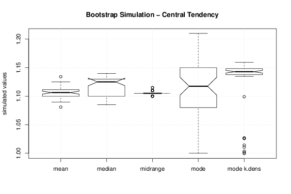
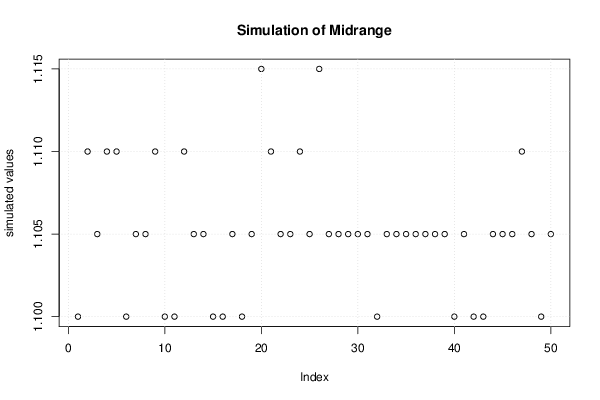
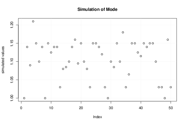
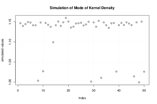
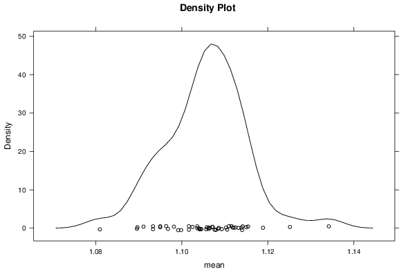
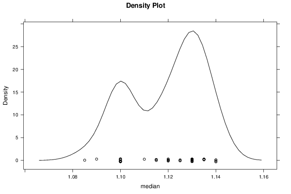
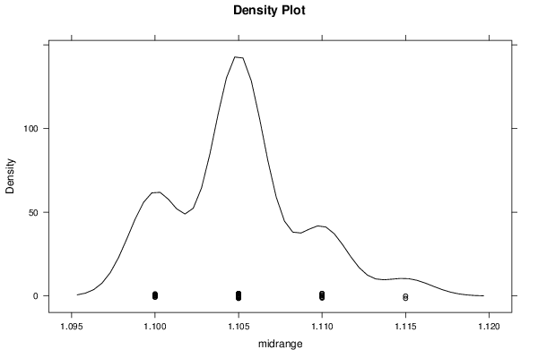
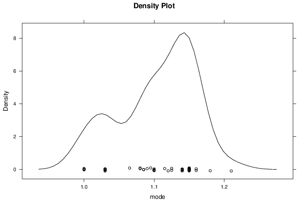
Title produced by software

Bootstrap Plot - Central Tendency

Date of computation

Sun, 25 Nov 2012 02:45:11 -0500

Cite this page as follows

Statistical Computations at FreeStatistics.org, Office for Research Development and Education, URL https://freestatistics.org/blog/index.php?v=date/2012/Nov/25/t1353829530jq99ryqyphroi5d.htm/, Retrieved Sun, 28 Apr 2024 19:11:49 +0000

Statistical Computations at FreeStatistics.org, Office for Research Development and Education, URL https://freestatistics.org/blog/index.php?pk=192551, Retrieved Sun, 28 Apr 2024 19:11:49 +0000

QR Codes:

Paste this QR Code to cite your computation.

Original text written by user:

IsPrivate?

No (this computation is public)

User-defined keywords

Estimated Impact

116

Family? (F = Feedback message, R = changed R code, M = changed R Module, P = changed Parameters, D = changed Data)

-     [Bootstrap Plot - Central Tendency] [] [2012-11-25 07:26:54] [74be16979710d4c4e7c6647856088456]
- R P   [Bootstrap Plot - Central Tendency] [] [2012-11-25 07:31:00] [74be16979710d4c4e7c6647856088456]
- R PD      [Bootstrap Plot - Central Tendency] [] [2012-11-25 07:45:11] [d41d8cd98f00b204e9800998ecf8427e] [Current]
- R PD        [Bootstrap Plot - Central Tendency] [] [2012-11-25 07:47:49] [74be16979710d4c4e7c6647856088456] 
-   P           [Bootstrap Plot - Central Tendency] [] [2012-11-25 07:51:52] [74be16979710d4c4e7c6647856088456] 

Feedback Forum

Post a new message

Dataseries X:

Download CSV

Histogram

Boxplots

Summary of computational transaction
Raw Input	view raw input (R code)
Raw Output	view raw output of R engine
Computing time	9 seconds
R Server	'Sir Maurice George Kendall' @ kendall.wessa.net

\begin{tabular}{lllllllll}
\hline
Summary of computational transaction \tabularnewline
Raw Input & view raw input (R code)  \tabularnewline
Raw Output & view raw output of R engine  \tabularnewline
Computing time & 9 seconds \tabularnewline
R Server & 'Sir Maurice George Kendall' @ kendall.wessa.net \tabularnewline
\hline
\end{tabular}
%Source: https://freestatistics.org/blog/index.php?pk=192551&T=0

[TABLE]
[ROW][C]Summary of computational transaction[/C][/ROW]
[ROW][C]Raw Input[/C][C]view raw input (R code) [/C][/ROW]
[ROW][C]Raw Output[/C][C]view raw output of R engine [/C][/ROW]
[ROW][C]Computing time[/C][C]9 seconds[/C][/ROW]
[ROW][C]R Server[/C][C]'Sir Maurice George Kendall' @ kendall.wessa.net[/C][/ROW]
[/TABLE]
Source: https://freestatistics.org/blog/index.php?pk=192551&T=0

Globally Unique Identifier (entire table): ba.freestatistics.org/blog/index.php?pk=192551&T=0

As an alternative you can also use a QR Code:

The GUIDs for individual cells are displayed in the table below:

Summary of computational transaction
Raw Input	view raw input (R code)
Raw Output	view raw output of R engine
Computing time	9 seconds
R Server	'Sir Maurice George Kendall' @ kendall.wessa.net

Estimation Results of Bootstrap
statistic	Q1	Estimate	Q3	S.D.	IQR
mean	1.1003	1.1078	1.1114	0.0093825	0.011076
median	1.1	1.13	1.13	0.015431	0.03
midrange	1.105	1.105	1.105	0.0037796	0
mode	1.08	1.09	1.15	0.05388	0.07
mode k.dens	1.1378	1.1457	1.1481	0.049129	0.010338

\begin{tabular}{lllllllll}
\hline
Estimation Results of Bootstrap \tabularnewline
statistic & Q1 & Estimate & Q3 & S.D. & IQR \tabularnewline
mean & 1.1003 & 1.1078 & 1.1114 & 0.0093825 & 0.011076 \tabularnewline
median & 1.1 & 1.13 & 1.13 & 0.015431 & 0.03 \tabularnewline
midrange & 1.105 & 1.105 & 1.105 & 0.0037796 & 0 \tabularnewline
mode & 1.08 & 1.09 & 1.15 & 0.05388 & 0.07 \tabularnewline
mode k.dens & 1.1378 & 1.1457 & 1.1481 & 0.049129 & 0.010338 \tabularnewline
\hline
\end{tabular}
%Source: https://freestatistics.org/blog/index.php?pk=192551&T=1

[TABLE]
[ROW][C]Estimation Results of Bootstrap[/C][/ROW]
[ROW][C]statistic[/C][C]Q1[/C][C]Estimate[/C][C]Q3[/C][C]S.D.[/C][C]IQR[/C][/ROW]
[ROW][C]mean[/C][C]1.1003[/C][C]1.1078[/C][C]1.1114[/C][C]0.0093825[/C][C]0.011076[/C][/ROW]
[ROW][C]median[/C][C]1.1[/C][C]1.13[/C][C]1.13[/C][C]0.015431[/C][C]0.03[/C][/ROW]
[ROW][C]midrange[/C][C]1.105[/C][C]1.105[/C][C]1.105[/C][C]0.0037796[/C][C]0[/C][/ROW]
[ROW][C]mode[/C][C]1.08[/C][C]1.09[/C][C]1.15[/C][C]0.05388[/C][C]0.07[/C][/ROW]
[ROW][C]mode k.dens[/C][C]1.1378[/C][C]1.1457[/C][C]1.1481[/C][C]0.049129[/C][C]0.010338[/C][/ROW]
[/TABLE]
Source: https://freestatistics.org/blog/index.php?pk=192551&T=1

Globally Unique Identifier (entire table): ba.freestatistics.org/blog/index.php?pk=192551&T=1

As an alternative you can also use a QR Code:

The GUIDs for individual cells are displayed in the table below:

Estimation Results of Bootstrap
statistic	Q1	Estimate	Q3	S.D.	IQR
mean	1.1003	1.1078	1.1114	0.0093825	0.011076
median	1.1	1.13	1.13	0.015431	0.03
midrange	1.105	1.105	1.105	0.0037796	0
mode	1.08	1.09	1.15	0.05388	0.07
mode k.dens	1.1378	1.1457	1.1481	0.049129	0.010338

Figure 1

PNG link

Postscript link

PDF link

Figure 2

PNG link

Postscript link

PDF link

Figure 3

PNG link

Postscript link

PDF link

Figure 4

PNG link

Postscript link

PDF link

Figure 5

PNG link

Postscript link

PDF link

Figure 6

PNG link

Postscript link

PDF link

Figure 7

PNG link

Postscript link

PDF link

Figure 8

PNG link

Postscript link

PDF link

Figure 9

PNG link

Postscript link

PDF link

Figure 10

PNG link

Postscript link

PDF link

Figure 11

PNG link

Postscript link

PDF link

Parameters (Session):

par1 = 50 ; par2 = 5 ; par3 = 0 ;

Parameters (R input):

par1 = 50 ; par2 = 5 ; par3 = 0 ;

R code (references can be found in the software module):

par3 <- '0'
par2 <- '5'
par1 <- '50'
par1 <- as.numeric(par1)
par2 <- as.numeric(par2)
if (par3 == '0') bw <- NULL
if (par3 != '0') bw <- as.numeric(par3)
if (par1 < 10) par1 = 10
if (par1 > 5000) par1 = 5000
library(modeest)
library(lattice)
library(boot)
boot.stat <- function(s,i)
{
s.mean <- mean(s[i])
s.median <- median(s[i])
s.midrange <- (max(s[i]) + min(s[i])) / 2
s.mode <- mlv(s[i], method='mfv')$M
s.kernelmode <- mlv(s[i], method='kernel', bw=bw)$M
c(s.mean, s.median, s.midrange, s.mode, s.kernelmode)
}
(r <- boot(x,boot.stat, R=par1, stype='i'))
bitmap(file='plot1.png')
plot(r$t[,1],type='p',ylab='simulated values',main='Simulation of Mean')
grid()
dev.off()
bitmap(file='plot2.png')
plot(r$t[,2],type='p',ylab='simulated values',main='Simulation of Median')
grid()
dev.off()
bitmap(file='plot3.png')
plot(r$t[,3],type='p',ylab='simulated values',main='Simulation of Midrange')
grid()
dev.off()
bitmap(file='plot7.png')
plot(r$t[,4],type='p',ylab='simulated values',main='Simulation of Mode')
grid()
dev.off()
bitmap(file='plot8.png')
plot(r$t[,5],type='p',ylab='simulated values',main='Simulation of Mode of Kernel Density')
grid()
dev.off()
bitmap(file='plot4.png')
densityplot(~r$t[,1],col='black',main='Density Plot',xlab='mean')
dev.off()
bitmap(file='plot5.png')
densityplot(~r$t[,2],col='black',main='Density Plot',xlab='median')
dev.off()
bitmap(file='plot6.png')
densityplot(~r$t[,3],col='black',main='Density Plot',xlab='midrange')
dev.off()
bitmap(file='plot9.png')
densityplot(~r$t[,4],col='black',main='Density Plot',xlab='mode')
dev.off()
bitmap(file='plot10.png')
densityplot(~r$t[,5],col='black',main='Density Plot',xlab='mode of kernel dens.')
dev.off()
z <- data.frame(cbind(r$t[,1],r$t[,2],r$t[,3],r$t[,4],r$t[,5]))
colnames(z) <- list('mean','median','midrange','mode','mode k.dens')
bitmap(file='plot11.png')
boxplot(z,notch=TRUE,ylab='simulated values',main='Bootstrap Simulation - Central Tendency')
grid()
dev.off()
load(file='createtable')
a<-table.start()
a<-table.row.start(a)
a<-table.element(a,'Estimation Results of Bootstrap',6,TRUE)
a<-table.row.end(a)
a<-table.row.start(a)
a<-table.element(a,'statistic',header=TRUE)
a<-table.element(a,'Q1',header=TRUE)
a<-table.element(a,'Estimate',header=TRUE)
a<-table.element(a,'Q3',header=TRUE)
a<-table.element(a,'S.D.',header=TRUE)
a<-table.element(a,'IQR',header=TRUE)
a<-table.row.end(a)
a<-table.row.start(a)
a<-table.element(a,'mean',header=TRUE)
q1 <- quantile(r$t[,1],0.25)[[1]]
q3 <- quantile(r$t[,1],0.75)[[1]]
a<-table.element(a,signif(q1,par2))
a<-table.element(a,signif(r$t0[1],par2))
a<-table.element(a,signif(q3,par2))
a<-table.element( a,signif( sqrt(var(r$t[,1])),par2 ) )
a<-table.element(a,signif(q3-q1,par2))
a<-table.row.end(a)
a<-table.row.start(a)
a<-table.element(a,'median',header=TRUE)
q1 <- quantile(r$t[,2],0.25)[[1]]
q3 <- quantile(r$t[,2],0.75)[[1]]
a<-table.element(a,signif(q1,par2))
a<-table.element(a,signif(r$t0[2],par2))
a<-table.element(a,signif(q3,par2))
a<-table.element(a,signif(sqrt(var(r$t[,2])),par2))
a<-table.element(a,signif(q3-q1,par2))
a<-table.row.end(a)
a<-table.row.start(a)
a<-table.element(a,'midrange',header=TRUE)
q1 <- quantile(r$t[,3],0.25)[[1]]
q3 <- quantile(r$t[,3],0.75)[[1]]
a<-table.element(a,signif(q1,par2))
a<-table.element(a,signif(r$t0[3],par2))
a<-table.element(a,signif(q3,par2))
a<-table.element(a,signif(sqrt(var(r$t[,3])),par2))
a<-table.element(a,signif(q3-q1,par2))
a<-table.row.end(a)
a<-table.row.start(a)
a<-table.element(a,'mode',header=TRUE)
q1 <- quantile(r$t[,4],0.25)[[1]]
q3 <- quantile(r$t[,4],0.75)[[1]]
a<-table.element(a,signif(q1,par2))
a<-table.element(a,signif(r$t0[4],par2))
a<-table.element(a,signif(q3,par2))
a<-table.element(a,signif(sqrt(var(r$t[,4])),par2))
a<-table.element(a,signif(q3-q1,par2))
a<-table.row.end(a)
a<-table.row.start(a)
a<-table.element(a,'mode k.dens',header=TRUE)
q1 <- quantile(r$t[,5],0.25)[[1]]
q3 <- quantile(r$t[,5],0.75)[[1]]
a<-table.element(a,signif(q1,par2))
a<-table.element(a,signif(r$t0[5],par2))
a<-table.element(a,signif(q3,par2))
a<-table.element(a,signif(sqrt(var(r$t[,5])),par2))
a<-table.element(a,signif(q3-q1,par2))
a<-table.row.end(a)
a<-table.end(a)
table.save(a,file='mytable.tab')

Free Statistics

Description of Statistical Computation

Tree of Dependent Computations

Dataset

Tables (Output of Computation)

Figures (Output of Computation)

Input Parameters & R Code