Free Statistics
of Irreproducible Research!
Description of Statistical Computation | |||||||||||||||||||||
|---|---|---|---|---|---|---|---|---|---|---|---|---|---|---|---|---|---|---|---|---|---|
| Author's title | |||||||||||||||||||||
| Author | *The author of this computation has been verified* | ||||||||||||||||||||
| R Software Module | rwasp_meanplot.wasp | ||||||||||||||||||||
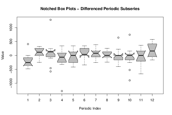
| Title produced by software | Mean Plot | ||||||||||||||||||||
| Date of computation | Tue, 02 Oct 2012 06:02:25 -0400 | ||||||||||||||||||||
| Cite this page as follows | Statistical Computations at FreeStatistics.org, Office for Research Development and Education, URL https://freestatistics.org/blog/index.php?v=date/2012/Oct/02/t1349172173rl8u57pixpaxgsp.htm/, Retrieved Sat, 04 May 2024 22:52:38 +0000 | ||||||||||||||||||||
| Statistical Computations at FreeStatistics.org, Office for Research Development and Education, URL https://freestatistics.org/blog/index.php?pk=171076, Retrieved Sat, 04 May 2024 22:52:38 +0000 | |||||||||||||||||||||
| QR Codes: | |||||||||||||||||||||
|
| |||||||||||||||||||||
| Original text written by user: | |||||||||||||||||||||
| IsPrivate? | No (this computation is public) | ||||||||||||||||||||
| User-defined keywords | |||||||||||||||||||||
| Estimated Impact | 68 | ||||||||||||||||||||
Tree of Dependent Computations | |||||||||||||||||||||
| Family? (F = Feedback message, R = changed R code, M = changed R Module, P = changed Parameters, D = changed Data) | |||||||||||||||||||||
| F [Univariate Data Series] [HPC Retail Sales] [2008-03-02 15:42:48] [74be16979710d4c4e7c6647856088456] - RMPD [Mean Plot] [With task 7] [2012-10-02 10:02:25] [af500d8a3ad66c35fc813daefbed0920] [Current] | |||||||||||||||||||||
| Feedback Forum | |||||||||||||||||||||
Post a new message | |||||||||||||||||||||
Dataset | |||||||||||||||||||||
| Dataseries X: | |||||||||||||||||||||
1280 1024 1120 1024 1280 1280 1280 1024 1280 1280 1280 1280 1280 1688 1440 1600 1280 1280 1280 1176 1280 1503 1440 1366 1280 1024 1280 2560 1280 1024 1280 1280 1440 1280 1440 1024 1440 1143 1280 1440 1280 1366 1024 1408 1366 1176 1920 1257 1280 1280 1440 1680 1440 1024 1140 1280 1280 1280 1280 1280 1440 1280 1152 1280 1280 1440 1280 1280 1440 1280 1280 1440 1280 1280 1600 1024 1366 1280 1280 1440 1366 1280 1024 1280 1440 1280 1280 1408 1280 1600 1600 1680 1440 1440 917 1280 1760 1280 1280 1280 1024 1366 1440 1280 1280 1920 1024 1024 1600 1117 1440 983 1024 1024 1280 1440 1280 1280 1280 1440 1280 1024 1024 1152 1280 1024 1366 1680 1680 1280 1366 1024 1440 1024 1280 1280 1280 1024 1280 | |||||||||||||||||||||
Tables (Output of Computation) | |||||||||||||||||||||
| |||||||||||||||||||||
Figures (Output of Computation) | |||||||||||||||||||||
Input Parameters & R Code | |||||||||||||||||||||
| Parameters (Session): | |||||||||||||||||||||
| Parameters (R input): | |||||||||||||||||||||
| par1 = 12 ; | |||||||||||||||||||||
| R code (references can be found in the software module): | |||||||||||||||||||||
par1 <- '12' | |||||||||||||||||||||