Free Statistics
of Irreproducible Research!
Description of Statistical Computation | |||||||||||||||||||||
|---|---|---|---|---|---|---|---|---|---|---|---|---|---|---|---|---|---|---|---|---|---|
| Author's title | |||||||||||||||||||||
| Author | *Unverified author* | ||||||||||||||||||||
| R Software Module | rwasp_sdplot.wasp | ||||||||||||||||||||
| Title produced by software | Standard Deviation Plot | ||||||||||||||||||||
| Date of computation | Tue, 13 Aug 2013 12:22:42 -0400 | ||||||||||||||||||||
| Cite this page as follows | Statistical Computations at FreeStatistics.org, Office for Research Development and Education, URL https://freestatistics.org/blog/index.php?v=date/2013/Aug/13/t1376413444pjdkhmm1sb2ppnr.htm/, Retrieved Thu, 02 May 2024 15:48:28 +0000 | ||||||||||||||||||||
| Statistical Computations at FreeStatistics.org, Office for Research Development and Education, URL https://freestatistics.org/blog/index.php?pk=211077, Retrieved Thu, 02 May 2024 15:48:28 +0000 | |||||||||||||||||||||
| QR Codes: | |||||||||||||||||||||
|
| |||||||||||||||||||||
| Original text written by user: | |||||||||||||||||||||
| IsPrivate? | No (this computation is public) | ||||||||||||||||||||
| User-defined keywords | |||||||||||||||||||||
| Estimated Impact | 162 | ||||||||||||||||||||
Tree of Dependent Computations | |||||||||||||||||||||
| Family? (F = Feedback message, R = changed R code, M = changed R Module, P = changed Parameters, D = changed Data) | |||||||||||||||||||||
| - [(Partial) Autocorrelation Function] [Stap 20/1] [2013-08-13 15:10:40] [9b490dd2ab715f1b5bf65aa31d98df3d] - RMP [Standard Deviation Plot] [stap 23 /1] [2013-08-13 16:22:42] [38a0db91cd47487c7649642dcb33e029] [Current] | |||||||||||||||||||||
| Feedback Forum | |||||||||||||||||||||
Post a new message | |||||||||||||||||||||
Dataset | |||||||||||||||||||||
| Dataseries X: | |||||||||||||||||||||
57 56 55 53 73 72 57 47 48 48 49 51 45 39 34 34 53 55 40 22 31 31 39 43 42 31 37 35 52 48 31 19 30 34 37 41 32 25 28 29 56 56 41 39 45 42 50 60 62 48 44 40 67 69 64 69 68 60 69 79 83 71 63 69 95 103 101 105 104 94 111 116 122 103 96 104 124 141 137 137 139 132 150 150 147 130 133 135 148 165 153 159 154 151 174 169 162 152 162 167 173 181 173 178 172 171 196 199 190 176 188 193 200 209 200 207 204 192 216 216 | |||||||||||||||||||||
Tables (Output of Computation) | |||||||||||||||||||||
| |||||||||||||||||||||
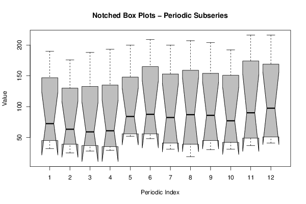
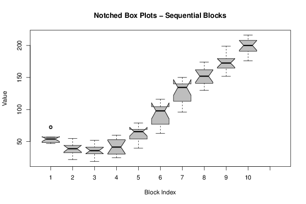
Figures (Output of Computation) | |||||||||||||||||||||
Input Parameters & R Code | |||||||||||||||||||||
| Parameters (Session): | |||||||||||||||||||||
| par1 = 12 ; | |||||||||||||||||||||
| Parameters (R input): | |||||||||||||||||||||
| par1 = 12 ; | |||||||||||||||||||||
| R code (references can be found in the software module): | |||||||||||||||||||||
par1 <- as.numeric(par1) | |||||||||||||||||||||