Free Statistics
of Irreproducible Research!
Description of Statistical Computation | |||||||||||||||||||||||||||||||||||||||||||||||||||||||||||||||||||||||||||||||||
|---|---|---|---|---|---|---|---|---|---|---|---|---|---|---|---|---|---|---|---|---|---|---|---|---|---|---|---|---|---|---|---|---|---|---|---|---|---|---|---|---|---|---|---|---|---|---|---|---|---|---|---|---|---|---|---|---|---|---|---|---|---|---|---|---|---|---|---|---|---|---|---|---|---|---|---|---|---|---|---|---|---|
| Author's title | |||||||||||||||||||||||||||||||||||||||||||||||||||||||||||||||||||||||||||||||||
| Author | *Unverified author* | ||||||||||||||||||||||||||||||||||||||||||||||||||||||||||||||||||||||||||||||||
| R Software Module | rwasp_bootstrapplot.wasp | ||||||||||||||||||||||||||||||||||||||||||||||||||||||||||||||||||||||||||||||||
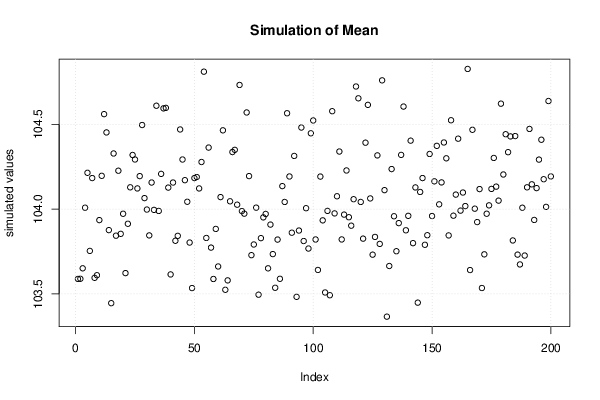
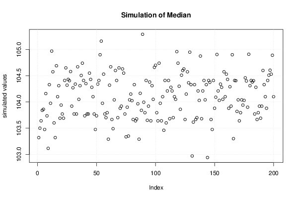
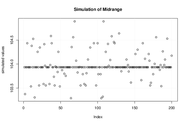
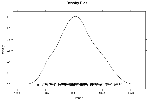
| Title produced by software | Blocked Bootstrap Plot - Central Tendency | ||||||||||||||||||||||||||||||||||||||||||||||||||||||||||||||||||||||||||||||||
| Date of computation | Tue, 08 Jan 2013 19:41:16 -0500 | ||||||||||||||||||||||||||||||||||||||||||||||||||||||||||||||||||||||||||||||||
| Cite this page as follows | Statistical Computations at FreeStatistics.org, Office for Research Development and Education, URL https://freestatistics.org/blog/index.php?v=date/2013/Jan/08/t13576921247y60zemn9yx3u6n.htm/, Retrieved Fri, 04 Jul 2025 08:29:31 +0000 | ||||||||||||||||||||||||||||||||||||||||||||||||||||||||||||||||||||||||||||||||
| Statistical Computations at FreeStatistics.org, Office for Research Development and Education, URL https://freestatistics.org/blog/index.php?pk=205090, Retrieved Fri, 04 Jul 2025 08:29:31 +0000 | |||||||||||||||||||||||||||||||||||||||||||||||||||||||||||||||||||||||||||||||||
| QR Codes: | |||||||||||||||||||||||||||||||||||||||||||||||||||||||||||||||||||||||||||||||||
|
| |||||||||||||||||||||||||||||||||||||||||||||||||||||||||||||||||||||||||||||||||
| Original text written by user: | |||||||||||||||||||||||||||||||||||||||||||||||||||||||||||||||||||||||||||||||||
| IsPrivate? | No (this computation is public) | ||||||||||||||||||||||||||||||||||||||||||||||||||||||||||||||||||||||||||||||||
| User-defined keywords | |||||||||||||||||||||||||||||||||||||||||||||||||||||||||||||||||||||||||||||||||
| Estimated Impact | 205 | ||||||||||||||||||||||||||||||||||||||||||||||||||||||||||||||||||||||||||||||||
Tree of Dependent Computations | |||||||||||||||||||||||||||||||||||||||||||||||||||||||||||||||||||||||||||||||||
| Family? (F = Feedback message, R = changed R code, M = changed R Module, P = changed Parameters, D = changed Data) | |||||||||||||||||||||||||||||||||||||||||||||||||||||||||||||||||||||||||||||||||
| - [Harrell-Davis Quantiles] [Opgave 4 oef 1 st...] [2013-01-08 17:32:56] [1d73611e45a05aa2060be114fa39c596] - R D [Harrell-Davis Quantiles] [Opgave 4 oef 2 st...] [2013-01-08 17:53:10] [1d73611e45a05aa2060be114fa39c596] - RMPD [Central Tendency] [Opgave 5 Oef 1 st...] [2013-01-08 18:52:58] [1d73611e45a05aa2060be114fa39c596] - RMPD [Univariate Data Series] [Opgave 6 Oef 1 st...] [2013-01-08 20:12:04] [1d73611e45a05aa2060be114fa39c596] - RMP [(Partial) Autocorrelation Function] [Opgave 6 oef 1 st...] [2013-01-08 21:23:13] [1d73611e45a05aa2060be114fa39c596] - P [(Partial) Autocorrelation Function] [Opgave 6 bis oef ...] [2013-01-08 21:46:39] [1d73611e45a05aa2060be114fa39c596] - RMPD [Blocked Bootstrap Plot - Central Tendency] [opgave 7 oef 2 de...] [2013-01-09 00:41:16] [40325e7317026cf0d36242170f65df44] [Current] | |||||||||||||||||||||||||||||||||||||||||||||||||||||||||||||||||||||||||||||||||
| Feedback Forum | |||||||||||||||||||||||||||||||||||||||||||||||||||||||||||||||||||||||||||||||||
Post a new message | |||||||||||||||||||||||||||||||||||||||||||||||||||||||||||||||||||||||||||||||||
Dataset | |||||||||||||||||||||||||||||||||||||||||||||||||||||||||||||||||||||||||||||||||
| Dataseries X: | |||||||||||||||||||||||||||||||||||||||||||||||||||||||||||||||||||||||||||||||||
101.81 101.72 101.78 102.04 102.36 102.56 102.69 102.77 102.85 102.9 102.72 102.79 102.9 102.91 103.29 103.35 102.97 103.05 103.18 103.21 103.32 103.31 103.6 103.68 103.77 103.82 103.86 103.9 103.63 103.65 103.7 103.77 103.94 104.03 104.03 104.29 104.35 104.67 104.73 104.86 104.05 104.15 104.27 104.33 104.41 104.4 104.41 104.6 104.61 104.65 104.55 104.51 104.74 104.89 104.91 104.93 104.95 104.97 105.16 105.29 105.35 105.36 105.45 105.3 105.73 105.86 105.85 105.95 105.97 106.15 105.37 105.39 | |||||||||||||||||||||||||||||||||||||||||||||||||||||||||||||||||||||||||||||||||
Tables (Output of Computation) | |||||||||||||||||||||||||||||||||||||||||||||||||||||||||||||||||||||||||||||||||
| |||||||||||||||||||||||||||||||||||||||||||||||||||||||||||||||||||||||||||||||||
Figures (Output of Computation) | |||||||||||||||||||||||||||||||||||||||||||||||||||||||||||||||||||||||||||||||||
Input Parameters & R Code | |||||||||||||||||||||||||||||||||||||||||||||||||||||||||||||||||||||||||||||||||
| Parameters (Session): | |||||||||||||||||||||||||||||||||||||||||||||||||||||||||||||||||||||||||||||||||
| par1 = Inschrijvingen nieuwe personenwagens (maandelijks) ; par2 = Excelbestand BlackBoard ; par3 = Maandelijkse gegevens van inschrijvingen nieuwe personenwagens van begin 2000 tot eind 2005 ; par4 = 12 ; | |||||||||||||||||||||||||||||||||||||||||||||||||||||||||||||||||||||||||||||||||
| Parameters (R input): | |||||||||||||||||||||||||||||||||||||||||||||||||||||||||||||||||||||||||||||||||
| par1 = 200 ; par2 = 12 ; | |||||||||||||||||||||||||||||||||||||||||||||||||||||||||||||||||||||||||||||||||
| R code (references can be found in the software module): | |||||||||||||||||||||||||||||||||||||||||||||||||||||||||||||||||||||||||||||||||
par2 <- '12' | |||||||||||||||||||||||||||||||||||||||||||||||||||||||||||||||||||||||||||||||||