Free Statistics

of Irreproducible Research!

Author's title

Author*Unverified author*
R Software Modulerwasp_meanversusmedian.wasp
Title produced by softwareMean versus Median
Date of computationMon, 04 Mar 2013 13:53:28 -0500
Cite this page as followsStatistical Computations at FreeStatistics.org, Office for Research Development and Education, URL https://freestatistics.org/blog/index.php?v=date/2013/Mar/04/t1362423279wtbw9gfkh1xp3jg.htm/, Retrieved Sun, 28 Apr 2024 00:32:07 +0000
Statistical Computations at FreeStatistics.org, Office for Research Development and Education, URL https://freestatistics.org/blog/index.php?pk=207334, Retrieved Sun, 28 Apr 2024 00:32:07 +0000
QR Codes:

Original text written by user:
IsPrivate?No (this computation is public)
User-defined keywords
Estimated Impact96
Family? (F = Feedback message, R = changed R code, M = changed R Module, P = changed Parameters, D = changed Data)
-     [Central Tendency] [] [2013-03-04 18:36:16] [d55d05654abdb5022ac9ec4fde0d976a]
- RM D    [Mean versus Median] [] [2013-03-04 18:53:28] [54665deafd3402f8325c0d656ab7be45] [Current]
Feedback Forum

Post a new message
Dataseries X:
369.82
373.1
374.55
375.01
374.81
375.31
375.31
375.39
375.59
376.26
377.18
377.26
377.26
381.87
387.09
387.14
388.78
389.16
389.16
389.42
389.49
388.97
388.97
389.09
389.09
391.76
390.96
391.76
392.8
393.06
393.06
393.26
393.87
394.47
394.57
394.57
394.57
399.57
406.13
407.03
409.46
409.9
409.9
410.14
410.54
410.69
410.79
410.97
410.97
413.8
423.31
423.85
426.6
426.26
426.26
426.32
427.14
427.55
428.29
428.8
428.8
434.87
435.66
440.75
440.99
441.04
441.04
441.88
441.92
442.48
442.81
442.81


Summary of computational transaction
Raw Inputview raw input (R code)
Raw Outputview raw output of R engine
Computing time1 seconds
R Server'Herman Ole Andreas Wold' @ wold.wessa.net

\begin{tabular}{lllllllll}
\hline
Summary of computational transaction \tabularnewline
Raw Input & view raw input (R code)  \tabularnewline
Raw Output & view raw output of R engine  \tabularnewline
Computing time & 1 seconds \tabularnewline
R Server & 'Herman Ole Andreas Wold' @ wold.wessa.net \tabularnewline
\hline
\end{tabular}
%Source: https://freestatistics.org/blog/index.php?pk=207334&T=0

[TABLE]
[ROW][C]Summary of computational transaction[/C][/ROW]
[ROW][C]Raw Input[/C][C]view raw input (R code) [/C][/ROW]
[ROW][C]Raw Output[/C][C]view raw output of R engine [/C][/ROW]
[ROW][C]Computing time[/C][C]1 seconds[/C][/ROW]
[ROW][C]R Server[/C][C]'Herman Ole Andreas Wold' @ wold.wessa.net[/C][/ROW]
[/TABLE]
Source: https://freestatistics.org/blog/index.php?pk=207334&T=0

Globally Unique Identifier (entire table): ba.freestatistics.org/blog/index.php?pk=207334&T=0

As an alternative you can also use a QR Code:  

The GUIDs for individual cells are displayed in the table below:

Summary of computational transaction
Raw Inputview raw input (R code)
Raw Outputview raw output of R engine
Computing time1 seconds
R Server'Herman Ole Andreas Wold' @ wold.wessa.net


Median versus Mean
mean404.34875
median394.57

\begin{tabular}{lllllllll}
\hline
Median versus Mean \tabularnewline
mean & 404.34875 \tabularnewline
median & 394.57 \tabularnewline
\hline
\end{tabular}
%Source: https://freestatistics.org/blog/index.php?pk=207334&T=1

[TABLE]
[ROW][C]Median versus Mean[/C][/ROW]
[ROW][C]mean[/C][C]404.34875[/C][/ROW]
[ROW][C]median[/C][C]394.57[/C][/ROW]
[/TABLE]
Source: https://freestatistics.org/blog/index.php?pk=207334&T=1

Globally Unique Identifier (entire table): ba.freestatistics.org/blog/index.php?pk=207334&T=1

As an alternative you can also use a QR Code:  

The GUIDs for individual cells are displayed in the table below:

Median versus Mean
mean404.34875
median394.57


Parameters (Session):
Parameters (R input):
R code (references can be found in the software module):
library(Hmisc)
m <- mean(x)
e <- median(x)
bitmap(file='test1.png')
op <- par(mfrow=c(2,1))
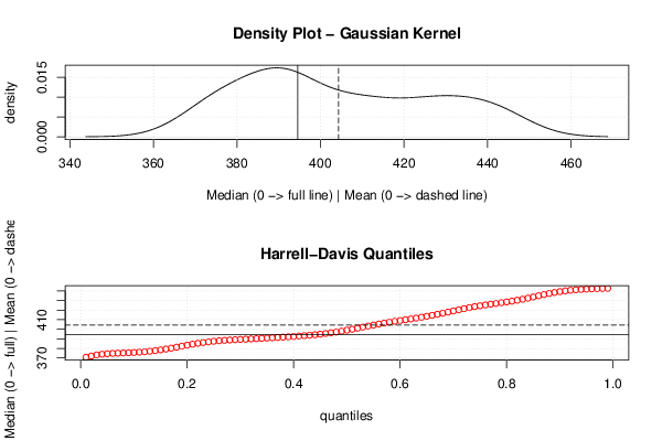
mydensity1 <- density(x,kernel='gaussian',na.rm=TRUE)
plot(mydensity1,main='Density Plot - Gaussian Kernel',xlab='Median (0 -> full line) | Mean (0 -> dashed line)',ylab='density')
abline(v=e,lty=1)
abline(v=m,lty=5)
grid()
myseq <- seq(0.01, 0.99, 0.01)
hd <- hdquantile(x, probs = myseq, se = TRUE, na.rm = FALSE, names = TRUE, weights=FALSE)
plot(myseq,hd,col=2,main='Harrell-Davis Quantiles',xlab='quantiles',ylab='Median (0 -> full) | Mean (0 -> dashed)')
abline(h=m,lty=5)
abline(h=e,lty=1)
grid()
par(op)
dev.off()
load(file='createtable')
a<-table.start()
a<-table.row.start(a)
a<-table.element(a,'Median versus Mean',2,TRUE)
a<-table.row.end(a)
a<-table.row.start(a)
a<-table.element(a,'mean',header=TRUE)
a<-table.element(a,mean(x))
a<-table.row.end(a)
a<-table.row.start(a)
a<-table.element(a,'median',header=TRUE)
a<-table.element(a,median(x))
a<-table.row.end(a)
a<-table.end(a)
table.save(a,file='mytable.tab')