Free Statistics
of Irreproducible Research!
Description of Statistical Computation | |||||||||||||||||||||
|---|---|---|---|---|---|---|---|---|---|---|---|---|---|---|---|---|---|---|---|---|---|
| Author's title | |||||||||||||||||||||
| Author | *Unverified author* | ||||||||||||||||||||
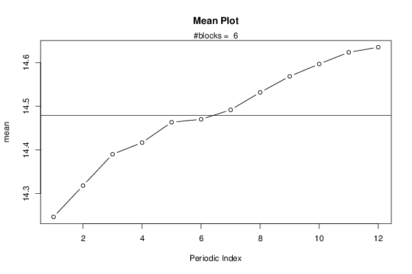
| R Software Module | rwasp_meanplot.wasp | ||||||||||||||||||||
| Title produced by software | Mean Plot | ||||||||||||||||||||
| Date of computation | Tue, 12 Mar 2013 10:38:02 -0400 | ||||||||||||||||||||
| Cite this page as follows | Statistical Computations at FreeStatistics.org, Office for Research Development and Education, URL https://freestatistics.org/blog/index.php?v=date/2013/Mar/12/t1363099745dsdqk75wabgfzt7.htm/, Retrieved Sun, 28 Apr 2024 18:54:37 +0000 | ||||||||||||||||||||
| Statistical Computations at FreeStatistics.org, Office for Research Development and Education, URL https://freestatistics.org/blog/index.php?pk=207727, Retrieved Sun, 28 Apr 2024 18:54:37 +0000 | |||||||||||||||||||||
| QR Codes: | |||||||||||||||||||||
|
| |||||||||||||||||||||
| Original text written by user: | |||||||||||||||||||||
| IsPrivate? | No (this computation is public) | ||||||||||||||||||||
| User-defined keywords | |||||||||||||||||||||
| Estimated Impact | 98 | ||||||||||||||||||||
Tree of Dependent Computations | |||||||||||||||||||||
| Family? (F = Feedback message, R = changed R code, M = changed R Module, P = changed Parameters, D = changed Data) | |||||||||||||||||||||
| - [Mean Plot] [] [2013-03-12 14:38:02] [5b48cba8ffed7710e2defc0d8d22bd89] [Current] | |||||||||||||||||||||
| Feedback Forum | |||||||||||||||||||||
Post a new message | |||||||||||||||||||||
Dataset | |||||||||||||||||||||
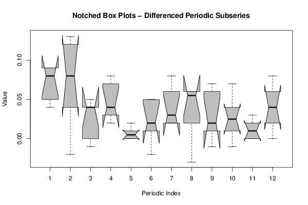
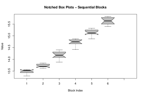
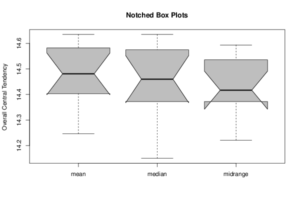
| Dataseries X: | |||||||||||||||||||||
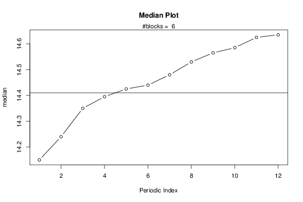
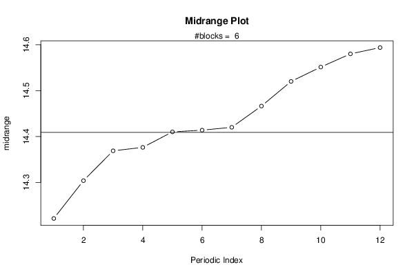
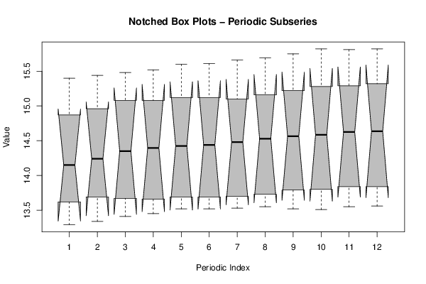
13,29 13,34 13,41 13,45 13,52 13,52 13,53 13,55 13,52 13,51 13,55 13,56 13,62 13,69 13,67 13,66 13,69 13,69 13,7 13,73 13,79 13,8 13,84 13,84 13,88 13,97 14,06 14,11 14,13 14,15 14,2 14,28 14,3 14,33 14,4 14,4 14,42 14,51 14,64 14,68 14,72 14,73 14,76 14,78 14,83 14,84 14,85 14,87 14,87 14,96 15,08 15,08 15,12 15,12 15,1 15,16 15,22 15,28 15,29 15,32 15,4 15,44 15,48 15,52 15,6 15,61 15,66 15,69 15,75 15,82 15,81 15,82 | |||||||||||||||||||||
Tables (Output of Computation) | |||||||||||||||||||||
| |||||||||||||||||||||
Figures (Output of Computation) | |||||||||||||||||||||
Input Parameters & R Code | |||||||||||||||||||||
| Parameters (Session): | |||||||||||||||||||||
| par1 = 12 ; | |||||||||||||||||||||
| Parameters (R input): | |||||||||||||||||||||
| par1 = 12 ; | |||||||||||||||||||||
| R code (references can be found in the software module): | |||||||||||||||||||||
par1 <- as.numeric(par1) | |||||||||||||||||||||