Free Statistics
of Irreproducible Research!
Description of Statistical Computation | |||||||||||||||||||||
|---|---|---|---|---|---|---|---|---|---|---|---|---|---|---|---|---|---|---|---|---|---|
| Author's title | |||||||||||||||||||||
| Author | *Unverified author* | ||||||||||||||||||||
| R Software Module | rwasp_meanplot.wasp | ||||||||||||||||||||
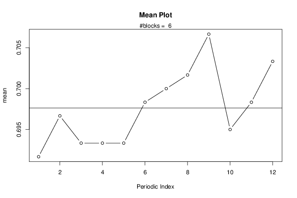
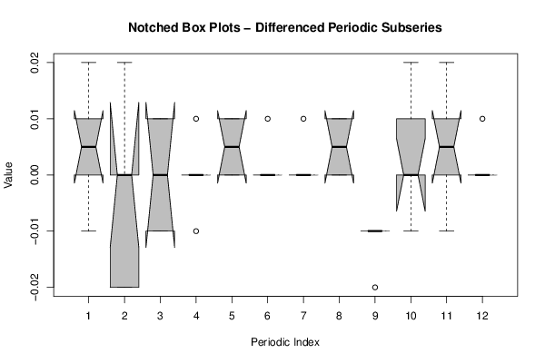
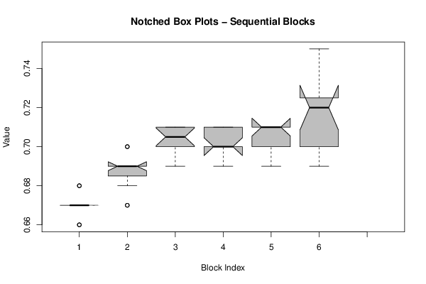
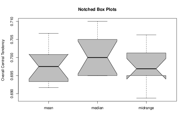
| Title produced by software | Mean Plot | ||||||||||||||||||||
| Date of computation | Tue, 12 Mar 2013 14:10:54 -0400 | ||||||||||||||||||||
| Cite this page as follows | Statistical Computations at FreeStatistics.org, Office for Research Development and Education, URL https://freestatistics.org/blog/index.php?v=date/2013/Mar/12/t1363111884optu6znp8ck7dz8.htm/, Retrieved Sun, 28 Apr 2024 20:13:15 +0000 | ||||||||||||||||||||
| Statistical Computations at FreeStatistics.org, Office for Research Development and Education, URL https://freestatistics.org/blog/index.php?pk=207743, Retrieved Sun, 28 Apr 2024 20:13:15 +0000 | |||||||||||||||||||||
| QR Codes: | |||||||||||||||||||||
|
| |||||||||||||||||||||
| Original text written by user: | |||||||||||||||||||||
| IsPrivate? | No (this computation is public) | ||||||||||||||||||||
| User-defined keywords | |||||||||||||||||||||
| Estimated Impact | 96 | ||||||||||||||||||||
Tree of Dependent Computations | |||||||||||||||||||||
| Family? (F = Feedback message, R = changed R code, M = changed R Module, P = changed Parameters, D = changed Data) | |||||||||||||||||||||
| - [Mean Plot] [Niet-gashoudend w...] [2013-03-12 18:10:54] [4772101fb1e8fea1eb9b6fc7ea4f009e] [Current] | |||||||||||||||||||||
| Feedback Forum | |||||||||||||||||||||
Post a new message | |||||||||||||||||||||
Dataset | |||||||||||||||||||||
| Dataseries X: | |||||||||||||||||||||
0,67 0,66 0,66 0,67 0,67 0,67 0,67 0,68 0,68 0,67 0,67 0,67 0,67 0,67 0,69 0,69 0,69 0,69 0,69 0,69 0,7 0,69 0,68 0,7 0,7 0,71 0,69 0,7 0,7 0,71 0,71 0,71 0,71 0,7 0,7 0,71 0,71 0,71 0,71 0,7 0,69 0,7 0,7 0,7 0,71 0,7 0,7 0,69 0,7 0,71 0,71 0,71 0,71 0,71 0,71 0,71 0,71 0,69 0,7 0,7 0,7 0,72 0,7 0,69 0,7 0,71 0,72 0,72 0,73 0,72 0,74 0,75 | |||||||||||||||||||||
Tables (Output of Computation) | |||||||||||||||||||||
| |||||||||||||||||||||
Figures (Output of Computation) | |||||||||||||||||||||
Input Parameters & R Code | |||||||||||||||||||||
| Parameters (Session): | |||||||||||||||||||||
| par1 = 12 ; | |||||||||||||||||||||
| Parameters (R input): | |||||||||||||||||||||
| par1 = 12 ; | |||||||||||||||||||||
| R code (references can be found in the software module): | |||||||||||||||||||||
par1 <- as.numeric(par1) | |||||||||||||||||||||