Free Statistics
of Irreproducible Research!
Description of Statistical Computation | |||||||||||||||||||||||||||||||||||||||||||||||||||||||||||||||||||||||||||||||||||||||||||||||||||||||||||||||||||||||||||||||||||||||||||||||||||||||||||||||||||||||||
|---|---|---|---|---|---|---|---|---|---|---|---|---|---|---|---|---|---|---|---|---|---|---|---|---|---|---|---|---|---|---|---|---|---|---|---|---|---|---|---|---|---|---|---|---|---|---|---|---|---|---|---|---|---|---|---|---|---|---|---|---|---|---|---|---|---|---|---|---|---|---|---|---|---|---|---|---|---|---|---|---|---|---|---|---|---|---|---|---|---|---|---|---|---|---|---|---|---|---|---|---|---|---|---|---|---|---|---|---|---|---|---|---|---|---|---|---|---|---|---|---|---|---|---|---|---|---|---|---|---|---|---|---|---|---|---|---|---|---|---|---|---|---|---|---|---|---|---|---|---|---|---|---|---|---|---|---|---|---|---|---|---|---|---|---|---|---|---|---|---|
| Author's title | |||||||||||||||||||||||||||||||||||||||||||||||||||||||||||||||||||||||||||||||||||||||||||||||||||||||||||||||||||||||||||||||||||||||||||||||||||||||||||||||||||||||||
| Author | *The author of this computation has been verified* | ||||||||||||||||||||||||||||||||||||||||||||||||||||||||||||||||||||||||||||||||||||||||||||||||||||||||||||||||||||||||||||||||||||||||||||||||||||||||||||||||||||||||
| R Software Module | rwasp_Simple Regression Y ~ X.wasp | ||||||||||||||||||||||||||||||||||||||||||||||||||||||||||||||||||||||||||||||||||||||||||||||||||||||||||||||||||||||||||||||||||||||||||||||||||||||||||||||||||||||||
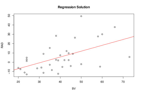
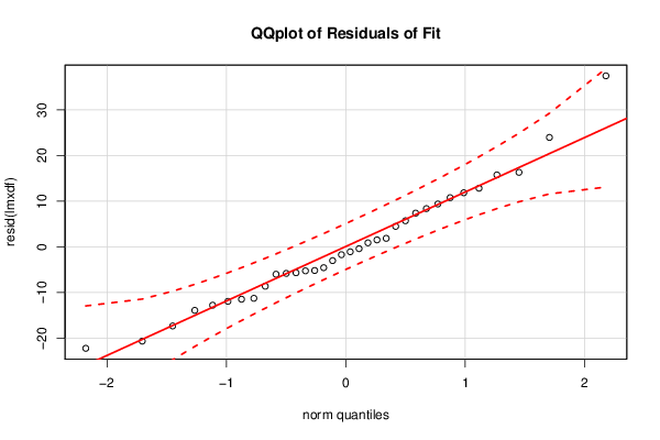
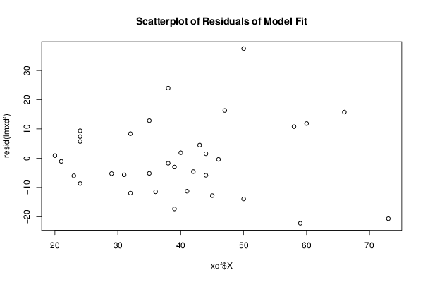
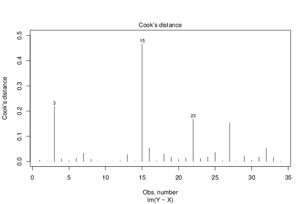
| Title produced by software | Simple Linear Regression | ||||||||||||||||||||||||||||||||||||||||||||||||||||||||||||||||||||||||||||||||||||||||||||||||||||||||||||||||||||||||||||||||||||||||||||||||||||||||||||||||||||||||
| Date of computation | Sat, 18 May 2013 07:35:15 -0400 | ||||||||||||||||||||||||||||||||||||||||||||||||||||||||||||||||||||||||||||||||||||||||||||||||||||||||||||||||||||||||||||||||||||||||||||||||||||||||||||||||||||||||
| Cite this page as follows | Statistical Computations at FreeStatistics.org, Office for Research Development and Education, URL https://freestatistics.org/blog/index.php?v=date/2013/May/18/t1368877055843e5r45i868xuy.htm/, Retrieved Sun, 28 Apr 2024 19:46:28 +0000 | ||||||||||||||||||||||||||||||||||||||||||||||||||||||||||||||||||||||||||||||||||||||||||||||||||||||||||||||||||||||||||||||||||||||||||||||||||||||||||||||||||||||||
| Statistical Computations at FreeStatistics.org, Office for Research Development and Education, URL https://freestatistics.org/blog/index.php?pk=209037, Retrieved Sun, 28 Apr 2024 19:46:28 +0000 | |||||||||||||||||||||||||||||||||||||||||||||||||||||||||||||||||||||||||||||||||||||||||||||||||||||||||||||||||||||||||||||||||||||||||||||||||||||||||||||||||||||||||
| QR Codes: | |||||||||||||||||||||||||||||||||||||||||||||||||||||||||||||||||||||||||||||||||||||||||||||||||||||||||||||||||||||||||||||||||||||||||||||||||||||||||||||||||||||||||
|
| |||||||||||||||||||||||||||||||||||||||||||||||||||||||||||||||||||||||||||||||||||||||||||||||||||||||||||||||||||||||||||||||||||||||||||||||||||||||||||||||||||||||||
| Original text written by user: | |||||||||||||||||||||||||||||||||||||||||||||||||||||||||||||||||||||||||||||||||||||||||||||||||||||||||||||||||||||||||||||||||||||||||||||||||||||||||||||||||||||||||
| IsPrivate? | No (this computation is public) | ||||||||||||||||||||||||||||||||||||||||||||||||||||||||||||||||||||||||||||||||||||||||||||||||||||||||||||||||||||||||||||||||||||||||||||||||||||||||||||||||||||||||
| User-defined keywords | |||||||||||||||||||||||||||||||||||||||||||||||||||||||||||||||||||||||||||||||||||||||||||||||||||||||||||||||||||||||||||||||||||||||||||||||||||||||||||||||||||||||||
| Estimated Impact | 412 | ||||||||||||||||||||||||||||||||||||||||||||||||||||||||||||||||||||||||||||||||||||||||||||||||||||||||||||||||||||||||||||||||||||||||||||||||||||||||||||||||||||||||
Tree of Dependent Computations | |||||||||||||||||||||||||||||||||||||||||||||||||||||||||||||||||||||||||||||||||||||||||||||||||||||||||||||||||||||||||||||||||||||||||||||||||||||||||||||||||||||||||
| Family? (F = Feedback message, R = changed R code, M = changed R Module, P = changed Parameters, D = changed Data) | |||||||||||||||||||||||||||||||||||||||||||||||||||||||||||||||||||||||||||||||||||||||||||||||||||||||||||||||||||||||||||||||||||||||||||||||||||||||||||||||||||||||||
| - [Simple Linear Regression] [RAD BPVT Regression] [2013-05-18 11:35:15] [a9208f4f8d3b118336aae915785f2bd9] [Current] - R D [Simple Linear Regression] [Stats exam prep -...] [2013-05-18 14:44:15] [a1457ae56ef989d68ac08bfda1bb63f0] - RMPD [Histogram, QQplot and Density] [Distribution plot...] [2013-05-18 15:41:29] [a1457ae56ef989d68ac08bfda1bb63f0] - R D [Histogram, QQplot and Density] [Distribution plot...] [2013-05-18 15:44:16] [a1457ae56ef989d68ac08bfda1bb63f0] - RMPD [Correlation] [exam correltion] [2013-05-18 16:50:10] [526987df82e09676a270245976380ec1] - RMPD [Histogram, QQplot and Density] [snmowqm] [2013-05-18 16:52:48] [526987df82e09676a270245976380ec1] - R D [Histogram, QQplot and Density] [+ve skew] [2013-05-18 16:54:47] [526987df82e09676a270245976380ec1] - RMPD [Correlation] [spearman exam data] [2013-05-18 16:55:26] [526987df82e09676a270245976380ec1] - RMPD [Histogram, QQplot and Density] [BPVT] [2013-05-21 17:10:37] [dd169dda621c71c4398ebb0f9fdc99bc] - RMPD [Two-Way ANOVA] [] [2013-05-21 19:08:47] [be0f7b6deff822c1e99df9393259f649] - RMPD [Histogram, QQplot and Density] [] [2013-05-21 19:58:30] [180e044edce56e655340260fe3c965df] - RMPD [Histogram, QQplot and Density] [] [2013-05-21 20:07:32] [180e044edce56e655340260fe3c965df] - RMPD [CARE Data - Boxplots and Scatterplot Matrix] [] [2013-05-21 20:13:43] [180e044edce56e655340260fe3c965df] - R D [Simple Linear Regression] [Males Simple Regr...] [2013-05-21 20:13:12] [274ef31908e26a640b7bd4e4d9070aea] - RMPD [Correlation] [] [2013-05-21 20:22:58] [180e044edce56e655340260fe3c965df] - R D [Simple Linear Regression] [] [2013-05-21 20:32:35] [1f91361365a675b598d66698e5c9b1fc] - M [Simple Linear Regression] [] [2013-05-21 20:41:23] [1f91361365a675b598d66698e5c9b1fc] - R D [Simple Linear Regression] [Female Simple Reg...] [2013-05-21 20:37:39] [1f91361365a675b598d66698e5c9b1fc] - R PD [Simple Linear Regression] [] [2013-05-21 21:28:08] [6877c1f985483048b09ba7926aa9573b] - RMP [Histogram, QQplot and Density] [test1] [2013-05-22 08:54:36] [45979429b8d230f66c17876d9d36ec0d] - R D [Simple Linear Regression] [] [2013-05-22 08:58:22] [14909ee9592b3303d106208bca5d4878] - RMPD [Correlation] [Male anf female r...] [2013-05-22 10:55:48] [32c5a5eecdcb56b653cfd8727ce24c34] - RM [Simple Linear Regression] [] [2013-05-22 13:07:44] [22aaafb3aaeb5140f0acb78bf4141f5b] - R [Simple Linear Regression] [Summer Exam Quest...] [2013-05-22 13:09:44] [a7ba1cea06fb99d1ea2d4dcded1ab41a] - R [Simple Linear Regression] [Regression - BPVT...] [2013-05-22 13:09:46] [a9284a28f46a6d49eba42780f57c79c3] - R [Simple Linear Regression] [Regression] [2013-05-22 13:11:05] [1da54e444dc2679e5d9aa3487bd18b49] - RM [Simple Linear Regression] [Linear regression...] [2013-05-22 13:10:51] [e11b7f6384dd13de42fda8812d748a63] - RM [Simple Linear Regression] [Rad and Bvpt regr...] [2013-05-22 13:11:44] [adf6e159a3755a825e40734540868e0e] - R [Simple Linear Regression] [Regression output...] [2013-05-22 13:11:34] [d348de2867ebac67b202b75ed3686d34] - [Simple Linear Regression] [Regression output...] [2013-05-22 13:46:58] [d348de2867ebac67b202b75ed3686d34] - RMPD [Histogram, QQplot and Density] [BOYS V GIRLS] [2013-05-22 14:16:28] [d348de2867ebac67b202b75ed3686d34] - RMPD [Histogram, QQplot and Density] [] [2013-05-22 14:27:44] [d348de2867ebac67b202b75ed3686d34] - RMPD [T-Tests] [Female and male r...] [2013-05-22 14:29:35] [d348de2867ebac67b202b75ed3686d34] - RMPD [] [Female rad scores] [-0001-11-30 00:00:00] [d348de2867ebac67b202b75ed3686d34] - RM [Simple Linear Regression] [RAD and BPVT Regr...] [2013-05-22 13:12:29] [2fa93cea200e9bacb3877c86c9d0fffb] - R [Simple Linear Regression] [Regression betwee...] [2013-05-22 13:12:33] [873a05c15549159fecd09e71c73360f4] - R [Simple Linear Regression] [blog 1.] [2013-05-22 13:12:40] [c3847fb9781c8af71938f4c7e4749741] - R [Simple Linear Regression] [June Exam ] [2013-05-22 13:12:50] [14909ee9592b3303d106208bca5d4878] - RMPD [Correlation] [Normality June exam] [2013-05-22 14:09:55] [14909ee9592b3303d106208bca5d4878] - RM [Simple Linear Regression] [q1 exam] [2013-05-22 13:13:05] [e9d96e04f324919fac52b0e4729a4aab] - R [Simple Linear Regression] [Linear regression...] [2013-05-22 13:12:44] [db051f6d419777365cfae0e3460cff71] - RM [Simple Linear Regression] [Question 2] [2013-05-22 13:13:21] [47982bab1b21f7e04987328ecb1c3458] - RMPD [CARE Data - Boxplots and Scatterplot Matrix] [] [2013-05-22 14:29:17] [47982bab1b21f7e04987328ecb1c3458] - RMPD [Histogram, QQplot and Density] [] [2013-05-22 14:40:28] [47982bab1b21f7e04987328ecb1c3458] - RMPD [Histogram, QQplot and Density] [] [2013-05-22 14:42:33] [47982bab1b21f7e04987328ecb1c3458] - RMPD [Histogram, QQplot and Density] [] [2013-05-22 14:45:39] [47982bab1b21f7e04987328ecb1c3458] - RMPD [MC Exam - Q11] [Hash Code] [2013-05-22 15:00:23] [47982bab1b21f7e04987328ecb1c3458] - R [Simple Linear Regression] [] [2013-05-22 13:13:58] [74be16979710d4c4e7c6647856088456] - R [Simple Linear Regression] [Summer exam 1] [2013-05-22 13:14:20] [5be6dfe262abe3b9e598f4c51751a54a] [Truncated] | |||||||||||||||||||||||||||||||||||||||||||||||||||||||||||||||||||||||||||||||||||||||||||||||||||||||||||||||||||||||||||||||||||||||||||||||||||||||||||||||||||||||||
| Feedback Forum | |||||||||||||||||||||||||||||||||||||||||||||||||||||||||||||||||||||||||||||||||||||||||||||||||||||||||||||||||||||||||||||||||||||||||||||||||||||||||||||||||||||||||
Post a new message | |||||||||||||||||||||||||||||||||||||||||||||||||||||||||||||||||||||||||||||||||||||||||||||||||||||||||||||||||||||||||||||||||||||||||||||||||||||||||||||||||||||||||
Dataset | |||||||||||||||||||||||||||||||||||||||||||||||||||||||||||||||||||||||||||||||||||||||||||||||||||||||||||||||||||||||||||||||||||||||||||||||||||||||||||||||||||||||||
| Dataseries X: | |||||||||||||||||||||||||||||||||||||||||||||||||||||||||||||||||||||||||||||||||||||||||||||||||||||||||||||||||||||||||||||||||||||||||||||||||||||||||||||||||||||||||
29 -6.5 21 -7.33 50 49.33 23 -11 35 -2.67 36 -8.33 47 26.33 32 9 38 2.67 44 9.67 46 9 42 2.33 39 -12.3 20 -6 73 5.67 38 28.33 43 12 50 -2 32 -11.3 24 1.33 24 3 59 -4.67 41 -5 24 -13 58 27.67 44 2.33 66 37.67 40 7.5 24 5 31 -5.67 45 -4 60 30 35 15.33 39 2 | |||||||||||||||||||||||||||||||||||||||||||||||||||||||||||||||||||||||||||||||||||||||||||||||||||||||||||||||||||||||||||||||||||||||||||||||||||||||||||||||||||||||||
Tables (Output of Computation) | |||||||||||||||||||||||||||||||||||||||||||||||||||||||||||||||||||||||||||||||||||||||||||||||||||||||||||||||||||||||||||||||||||||||||||||||||||||||||||||||||||||||||
| |||||||||||||||||||||||||||||||||||||||||||||||||||||||||||||||||||||||||||||||||||||||||||||||||||||||||||||||||||||||||||||||||||||||||||||||||||||||||||||||||||||||||
Figures (Output of Computation) | |||||||||||||||||||||||||||||||||||||||||||||||||||||||||||||||||||||||||||||||||||||||||||||||||||||||||||||||||||||||||||||||||||||||||||||||||||||||||||||||||||||||||
Input Parameters & R Code | |||||||||||||||||||||||||||||||||||||||||||||||||||||||||||||||||||||||||||||||||||||||||||||||||||||||||||||||||||||||||||||||||||||||||||||||||||||||||||||||||||||||||
| Parameters (Session): | |||||||||||||||||||||||||||||||||||||||||||||||||||||||||||||||||||||||||||||||||||||||||||||||||||||||||||||||||||||||||||||||||||||||||||||||||||||||||||||||||||||||||
| par1 = 2 ; par2 = 1 ; par3 = TRUE ; | |||||||||||||||||||||||||||||||||||||||||||||||||||||||||||||||||||||||||||||||||||||||||||||||||||||||||||||||||||||||||||||||||||||||||||||||||||||||||||||||||||||||||
| Parameters (R input): | |||||||||||||||||||||||||||||||||||||||||||||||||||||||||||||||||||||||||||||||||||||||||||||||||||||||||||||||||||||||||||||||||||||||||||||||||||||||||||||||||||||||||
| par1 = 2 ; par2 = 1 ; par3 = TRUE ; | |||||||||||||||||||||||||||||||||||||||||||||||||||||||||||||||||||||||||||||||||||||||||||||||||||||||||||||||||||||||||||||||||||||||||||||||||||||||||||||||||||||||||
| R code (references can be found in the software module): | |||||||||||||||||||||||||||||||||||||||||||||||||||||||||||||||||||||||||||||||||||||||||||||||||||||||||||||||||||||||||||||||||||||||||||||||||||||||||||||||||||||||||
par3 <- 'TRUE' | |||||||||||||||||||||||||||||||||||||||||||||||||||||||||||||||||||||||||||||||||||||||||||||||||||||||||||||||||||||||||||||||||||||||||||||||||||||||||||||||||||||||||