Free Statistics
of Irreproducible Research!
Description of Statistical Computation | |||||||||||||||||||||
|---|---|---|---|---|---|---|---|---|---|---|---|---|---|---|---|---|---|---|---|---|---|
| Author's title | |||||||||||||||||||||
| Author | *Unverified author* | ||||||||||||||||||||
| R Software Module | rwasp_meanplot.wasp | ||||||||||||||||||||
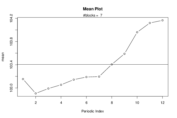
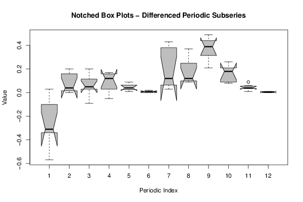
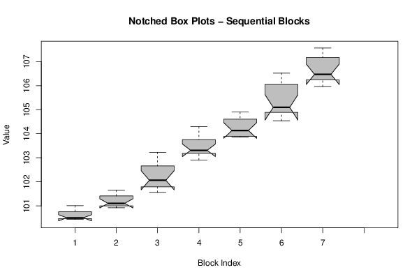
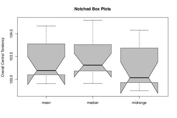
| Title produced by software | Mean Plot | ||||||||||||||||||||
| Date of computation | Mon, 14 Oct 2013 03:54:35 -0400 | ||||||||||||||||||||
| Cite this page as follows | Statistical Computations at FreeStatistics.org, Office for Research Development and Education, URL https://freestatistics.org/blog/index.php?v=date/2013/Oct/14/t1381737311awgdqykgqqpvl20.htm/, Retrieved Sun, 28 Apr 2024 06:45:35 +0000 | ||||||||||||||||||||
| Statistical Computations at FreeStatistics.org, Office for Research Development and Education, URL https://freestatistics.org/blog/index.php?pk=215376, Retrieved Sun, 28 Apr 2024 06:45:35 +0000 | |||||||||||||||||||||
| QR Codes: | |||||||||||||||||||||
|
| |||||||||||||||||||||
| Original text written by user: | |||||||||||||||||||||
| IsPrivate? | No (this computation is public) | ||||||||||||||||||||
| User-defined keywords | |||||||||||||||||||||
| Estimated Impact | 112 | ||||||||||||||||||||
Tree of Dependent Computations | |||||||||||||||||||||
| Family? (F = Feedback message, R = changed R code, M = changed R Module, P = changed Parameters, D = changed Data) | |||||||||||||||||||||
| - [Univariate Data Series] [] [2013-10-14 07:00:14] [9fb2675916b8773bb0a74f31adc60d44] - R PD [Univariate Data Series] [] [2013-10-14 07:09:20] [9fb2675916b8773bb0a74f31adc60d44] - RMPD [Mean Plot] [] [2013-10-14 07:50:36] [9fb2675916b8773bb0a74f31adc60d44] - R D [Mean Plot] [] [2013-10-14 07:54:35] [79b59004c90874912279e9b1431bd052] [Current] | |||||||||||||||||||||
| Feedback Forum | |||||||||||||||||||||
Post a new message | |||||||||||||||||||||
Dataset | |||||||||||||||||||||
| Dataseries X: | |||||||||||||||||||||
100,44 100,47 100,49 100,52 100,47 100,48 100,48 100,53 100,62 100,89 100,97 101,01 101,02 100,92 100,93 100,98 101,07 101,1 101,11 101,19 101,31 101,52 101,61 101,65 101,66 101,56 101,75 101,83 101,98 102,06 102,07 102,1 102,42 102,91 103,14 103,23 103,23 102,91 103,11 103,14 103,26 103,3 103,32 103,44 103,54 103,98 104,24 104,29 104,29 103,98 103,98 103,89 103,86 103,88 103,88 104,31 104,41 104,8 104,89 104,9 104,9 104,54 104,67 104,87 105,04 105,09 105,1 105,46 105,83 106,27 106,46 106,52 106,53 105,96 106 106,15 106,32 106,41 106,41 106,81 106,99 107,35 107,53 107,56 | |||||||||||||||||||||
Tables (Output of Computation) | |||||||||||||||||||||
| |||||||||||||||||||||
Figures (Output of Computation) | |||||||||||||||||||||
Input Parameters & R Code | |||||||||||||||||||||
| Parameters (Session): | |||||||||||||||||||||
| par1 = 12 ; | |||||||||||||||||||||
| Parameters (R input): | |||||||||||||||||||||
| par1 = 12 ; | |||||||||||||||||||||
| R code (references can be found in the software module): | |||||||||||||||||||||
par1 <- as.numeric(par1) | |||||||||||||||||||||