Free Statistics
of Irreproducible Research!
Description of Statistical Computation | |||||||||||||||||||||
|---|---|---|---|---|---|---|---|---|---|---|---|---|---|---|---|---|---|---|---|---|---|
| Author's title | |||||||||||||||||||||
| Author | *Unverified author* | ||||||||||||||||||||
| R Software Module | rwasp_meanplot.wasp | ||||||||||||||||||||
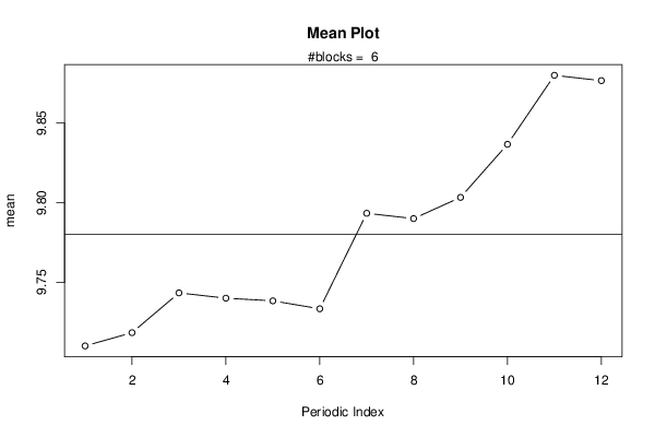
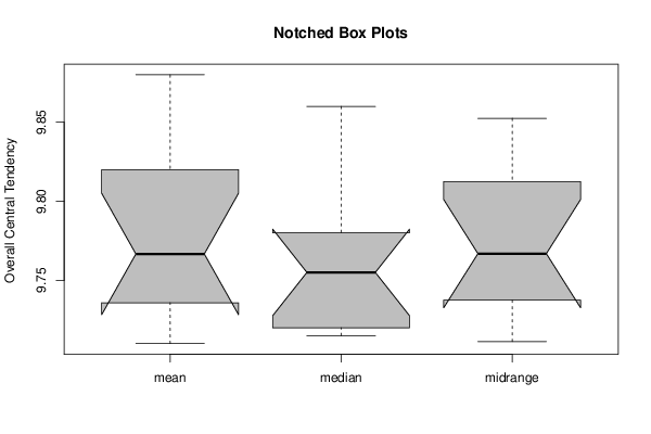
| Title produced by software | Mean Plot | ||||||||||||||||||||
| Date of computation | Mon, 14 Oct 2013 04:05:55 -0400 | ||||||||||||||||||||
| Cite this page as follows | Statistical Computations at FreeStatistics.org, Office for Research Development and Education, URL https://freestatistics.org/blog/index.php?v=date/2013/Oct/14/t1381738023sfq0jbek2qcwxya.htm/, Retrieved Sat, 27 Apr 2024 14:12:12 +0000 | ||||||||||||||||||||
| Statistical Computations at FreeStatistics.org, Office for Research Development and Education, URL https://freestatistics.org/blog/index.php?pk=215397, Retrieved Sat, 27 Apr 2024 14:12:12 +0000 | |||||||||||||||||||||
| QR Codes: | |||||||||||||||||||||
|
| |||||||||||||||||||||
| Original text written by user: | |||||||||||||||||||||
| IsPrivate? | No (this computation is public) | ||||||||||||||||||||
| User-defined keywords | |||||||||||||||||||||
| Estimated Impact | 105 | ||||||||||||||||||||
Tree of Dependent Computations | |||||||||||||||||||||
| Family? (F = Feedback message, R = changed R code, M = changed R Module, P = changed Parameters, D = changed Data) | |||||||||||||||||||||
| - [Mean Plot] [] [2013-10-14 08:05:55] [ccf63754fa7d22a76bdef567828ba364] [Current] | |||||||||||||||||||||
| Feedback Forum | |||||||||||||||||||||
Post a new message | |||||||||||||||||||||
Dataset | |||||||||||||||||||||
| Dataseries X: | |||||||||||||||||||||
9,27 9,30 9,35 9,33 9,37 9,42 9,45 9,38 9,40 9,43 9,45 9,49 9,47 9,48 9,52 9,53 9,53 9,54 9,57 9,61 9,61 9,63 9,64 9,60 9,64 9,66 9,67 9,70 9,72 9,73 9,77 9,72 9,68 9,62 9,79 9,77 9,79 9,77 9,78 9,81 9,74 9,70 9,78 9,85 9,83 9,90 9,93 9,85 9,95 9,97 10,02 9,97 9,95 9,95 9,98 10,00 10,04 10,05 10,06 10,09 10,14 10,13 10,12 10,10 10,12 10,06 10,21 10,18 10,26 10,39 10,41 10,46 | |||||||||||||||||||||
Tables (Output of Computation) | |||||||||||||||||||||
| |||||||||||||||||||||
Figures (Output of Computation) | |||||||||||||||||||||
Input Parameters & R Code | |||||||||||||||||||||
| Parameters (Session): | |||||||||||||||||||||
| par1 = 12 ; | |||||||||||||||||||||
| Parameters (R input): | |||||||||||||||||||||
| par1 = 12 ; | |||||||||||||||||||||
| R code (references can be found in the software module): | |||||||||||||||||||||
par1 <- as.numeric(par1) | |||||||||||||||||||||