Free Statistics
of Irreproducible Research!
Description of Statistical Computation | |||||||||||||||||||||||||||||||||
|---|---|---|---|---|---|---|---|---|---|---|---|---|---|---|---|---|---|---|---|---|---|---|---|---|---|---|---|---|---|---|---|---|---|
| Author's title | |||||||||||||||||||||||||||||||||
| Author | *Unverified author* | ||||||||||||||||||||||||||||||||
| R Software Module | rwasp_meanversusmedian.wasp | ||||||||||||||||||||||||||||||||
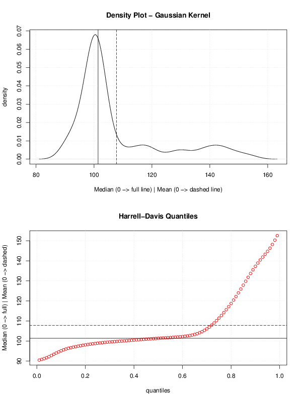
| Title produced by software | Mean versus Median | ||||||||||||||||||||||||||||||||
| Date of computation | Mon, 14 Oct 2013 06:23:45 -0400 | ||||||||||||||||||||||||||||||||
| Cite this page as follows | Statistical Computations at FreeStatistics.org, Office for Research Development and Education, URL https://freestatistics.org/blog/index.php?v=date/2013/Oct/14/t1381746463rhcbw4a6qhid6fj.htm/, Retrieved Sun, 28 Apr 2024 00:54:08 +0000 | ||||||||||||||||||||||||||||||||
| Statistical Computations at FreeStatistics.org, Office for Research Development and Education, URL https://freestatistics.org/blog/index.php?pk=215480, Retrieved Sun, 28 Apr 2024 00:54:08 +0000 | |||||||||||||||||||||||||||||||||
| QR Codes: | |||||||||||||||||||||||||||||||||
|
| |||||||||||||||||||||||||||||||||
| Original text written by user: | |||||||||||||||||||||||||||||||||
| IsPrivate? | No (this computation is public) | ||||||||||||||||||||||||||||||||
| User-defined keywords | |||||||||||||||||||||||||||||||||
| Estimated Impact | 99 | ||||||||||||||||||||||||||||||||
Tree of Dependent Computations | |||||||||||||||||||||||||||||||||
| Family? (F = Feedback message, R = changed R code, M = changed R Module, P = changed Parameters, D = changed Data) | |||||||||||||||||||||||||||||||||
| - [Central Tendency] [] [2013-10-14 08:50:17] [256d78ccaa024c70359216b2e3721f69] - RM D [Mean versus Median] [] [2013-10-14 10:23:45] [edfef9daf94f6afee2f7e041aec7fc2a] [Current] | |||||||||||||||||||||||||||||||||
| Feedback Forum | |||||||||||||||||||||||||||||||||
Post a new message | |||||||||||||||||||||||||||||||||
Dataset | |||||||||||||||||||||||||||||||||
| Dataseries X: | |||||||||||||||||||||||||||||||||
93.61 93.17 91.60 90.30 90.88 91.06 92.05 95.29 96.44 96.49 96.52 96.09 99.16 98.09 99.41 99.87 100.06 99.65 99.92 98.44 102.64 112.33 115.63 118.29 121.43 129.96 147.73 154.10 150.09 144.14 141.54 136.68 129.32 118.99 109.61 106.22 104.97 102.45 101.91 101.77 102.67 103.45 101.41 102.45 102.17 101.40 101.68 100.61 97.93 98.30 99.79 101.62 101.55 102.43 102.09 102.01 102.26 101.24 100.91 100.67 100.33 99.99 99.23 98.17 97.38 96.70 98.65 100.68 101.07 101.12 101.13 99.88 99.20 99.91 103.62 108.05 113.96 117.39 126.04 139.67 145.04 142.37 137.72 132.46 | |||||||||||||||||||||||||||||||||
Tables (Output of Computation) | |||||||||||||||||||||||||||||||||
| |||||||||||||||||||||||||||||||||
Figures (Output of Computation) | |||||||||||||||||||||||||||||||||
Input Parameters & R Code | |||||||||||||||||||||||||||||||||
| Parameters (Session): | |||||||||||||||||||||||||||||||||
| Parameters (R input): | |||||||||||||||||||||||||||||||||
| R code (references can be found in the software module): | |||||||||||||||||||||||||||||||||
library(Hmisc) | |||||||||||||||||||||||||||||||||