Free Statistics
of Irreproducible Research!
Description of Statistical Computation | |||||||||||||||||||||
|---|---|---|---|---|---|---|---|---|---|---|---|---|---|---|---|---|---|---|---|---|---|
| Author's title | |||||||||||||||||||||
| Author | *Unverified author* | ||||||||||||||||||||
| R Software Module | rwasp_meanplot.wasp | ||||||||||||||||||||
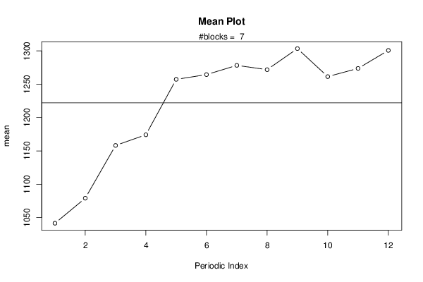
| Title produced by software | Mean Plot | ||||||||||||||||||||
| Date of computation | Wed, 16 Oct 2013 06:32:50 -0400 | ||||||||||||||||||||
| Cite this page as follows | Statistical Computations at FreeStatistics.org, Office for Research Development and Education, URL https://freestatistics.org/blog/index.php?v=date/2013/Oct/16/t138191959885729exq82kyjlh.htm/, Retrieved Sun, 28 Apr 2024 00:34:07 +0000 | ||||||||||||||||||||
| Statistical Computations at FreeStatistics.org, Office for Research Development and Education, URL https://freestatistics.org/blog/index.php?pk=216046, Retrieved Sun, 28 Apr 2024 00:34:07 +0000 | |||||||||||||||||||||
| QR Codes: | |||||||||||||||||||||
|
| |||||||||||||||||||||
| Original text written by user: | |||||||||||||||||||||
| IsPrivate? | No (this computation is public) | ||||||||||||||||||||
| User-defined keywords | |||||||||||||||||||||
| Estimated Impact | 109 | ||||||||||||||||||||
Tree of Dependent Computations | |||||||||||||||||||||
| Family? (F = Feedback message, R = changed R code, M = changed R Module, P = changed Parameters, D = changed Data) | |||||||||||||||||||||
| - [Mean Plot] [Reservepositie IM...] [2013-10-16 10:32:50] [a3fde7297e5409122ee2dd3b0c427a94] [Current] - R P [Mean Plot] [WLWZ1] [2013-10-19 09:57:06] [74be16979710d4c4e7c6647856088456] - R P [Mean Plot] [Reserve positie I...] [2013-10-19 10:00:35] [24038aabf47565f93cb94afd3d1da284] - R PD [Mean Plot] [WLWZ 4] [2013-10-19 10:04:43] [24038aabf47565f93cb94afd3d1da284] - R PD [Mean Plot] [WLWZ 52] [2013-10-19 10:07:28] [24038aabf47565f93cb94afd3d1da284] | |||||||||||||||||||||
| Feedback Forum | |||||||||||||||||||||
Post a new message | |||||||||||||||||||||
Dataset | |||||||||||||||||||||
| Dataseries X: | |||||||||||||||||||||
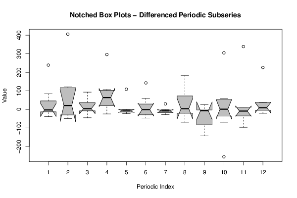
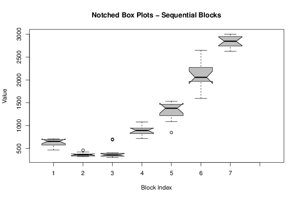
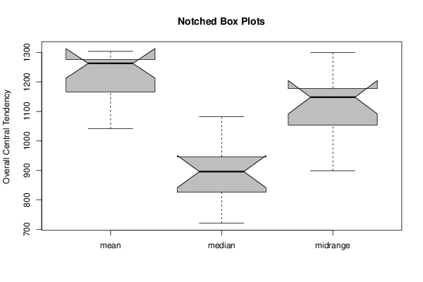
679 687 638 628 604 713 712 693 697 555 486 470 465 426 384 379 381 380 351 346 339 336 333 324 324 321 304 343 407 389 361 353 361 387 692 704 742 721 843 847 945 946 946 945 1082 1075 820 832 851 1090 1203 1239 1535 1527 1480 1452 1383 1381 1429 1376 1602 1597 2003 1958 1997 1986 2129 2115 2297 2250 2309 2648 2627 2711 2732 2825 2932 2910 2969 2999 2965 2846 2847 2751 | |||||||||||||||||||||
Tables (Output of Computation) | |||||||||||||||||||||
| |||||||||||||||||||||
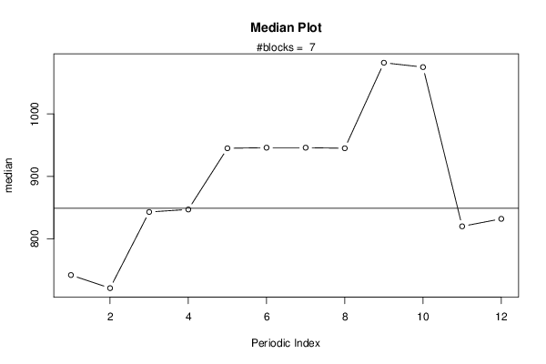
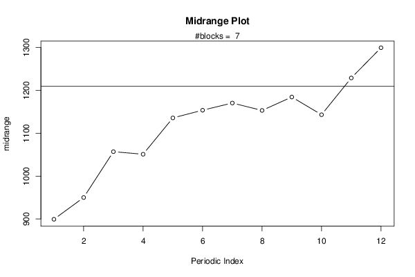
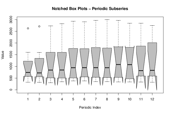
Figures (Output of Computation) | |||||||||||||||||||||
Input Parameters & R Code | |||||||||||||||||||||
| Parameters (Session): | |||||||||||||||||||||
| par1 = 12 ; | |||||||||||||||||||||
| Parameters (R input): | |||||||||||||||||||||
| par1 = 12 ; | |||||||||||||||||||||
| R code (references can be found in the software module): | |||||||||||||||||||||
par1 <- as.numeric(par1) | |||||||||||||||||||||