Free Statistics
of Irreproducible Research!
Description of Statistical Computation | |||||||||||||||||||||
|---|---|---|---|---|---|---|---|---|---|---|---|---|---|---|---|---|---|---|---|---|---|
| Author's title | |||||||||||||||||||||
| Author | *Unverified author* | ||||||||||||||||||||
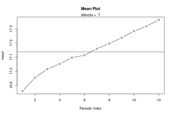
| R Software Module | rwasp_meanplot.wasp | ||||||||||||||||||||
| Title produced by software | Mean Plot | ||||||||||||||||||||
| Date of computation | Wed, 16 Oct 2013 13:24:02 -0400 | ||||||||||||||||||||
| Cite this page as follows | Statistical Computations at FreeStatistics.org, Office for Research Development and Education, URL https://freestatistics.org/blog/index.php?v=date/2013/Oct/16/t138194425502pxsd8ektkbuix.htm/, Retrieved Sun, 28 Apr 2024 11:00:07 +0000 | ||||||||||||||||||||
| Statistical Computations at FreeStatistics.org, Office for Research Development and Education, URL https://freestatistics.org/blog/index.php?pk=216214, Retrieved Sun, 28 Apr 2024 11:00:07 +0000 | |||||||||||||||||||||
| QR Codes: | |||||||||||||||||||||
|
| |||||||||||||||||||||
| Original text written by user: | |||||||||||||||||||||
| IsPrivate? | No (this computation is public) | ||||||||||||||||||||
| User-defined keywords | |||||||||||||||||||||
| Estimated Impact | 74 | ||||||||||||||||||||
Tree of Dependent Computations | |||||||||||||||||||||
| Family? (F = Feedback message, R = changed R code, M = changed R Module, P = changed Parameters, D = changed Data) | |||||||||||||||||||||
| - [Mean Plot] [] [2013-10-16 17:24:02] [1177af5e7ddeef06deae586abecaeb9d] [Current] | |||||||||||||||||||||
| Feedback Forum | |||||||||||||||||||||
Post a new message | |||||||||||||||||||||
Dataset | |||||||||||||||||||||
| Dataseries X: | |||||||||||||||||||||
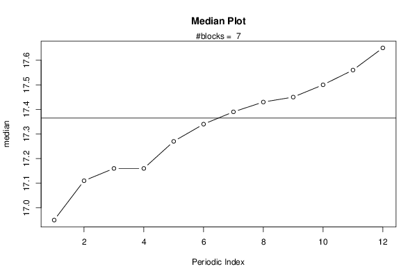
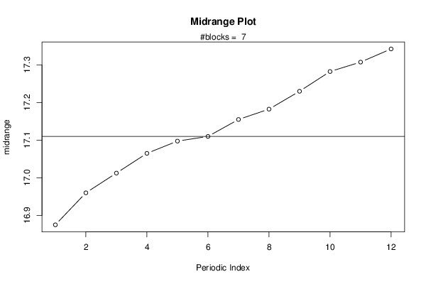
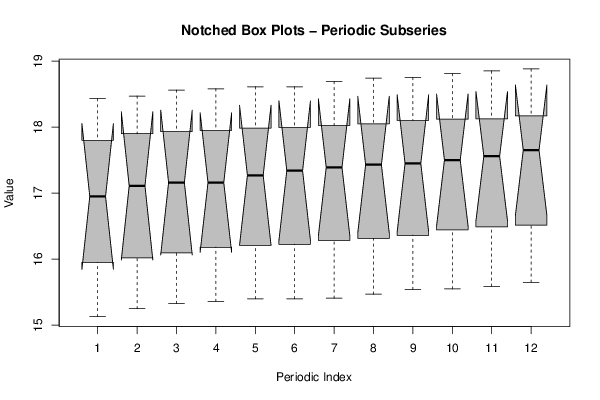
15,13 15,25 15,33 15,36 15,40 15,40 15,41 15,47 15,54 15,55 15,59 15,65 15,75 15,86 15,89 15,94 15,93 15,95 15,99 15,99 16,06 16,08 16,07 16,11 16,15 16,18 16,30 16,42 16,49 16,50 16,58 16,64 16,66 16,81 16,91 16,92 16,95 17,11 17,16 17,16 17,27 17,34 17,39 17,43 17,45 17,50 17,56 17,65 17,62 17,70 17,72 17,71 17,74 17,75 17,78 17,80 17,86 17,88 17,89 17,94 17,98 18,10 18,14 18,19 18,23 18,24 18,27 18,30 18,34 18,36 18,36 18,40 18,43 18,47 18,56 18,58 18,61 18,61 18,69 18,74 18,75 18,81 18,85 18,88 | |||||||||||||||||||||
Tables (Output of Computation) | |||||||||||||||||||||
| |||||||||||||||||||||
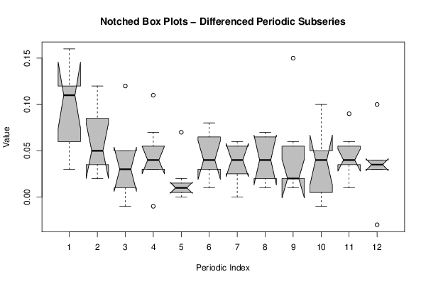
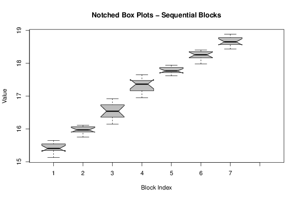
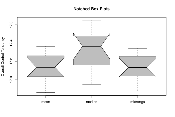
Figures (Output of Computation) | |||||||||||||||||||||
Input Parameters & R Code | |||||||||||||||||||||
| Parameters (Session): | |||||||||||||||||||||
| par1 = 12 ; | |||||||||||||||||||||
| Parameters (R input): | |||||||||||||||||||||
| par1 = 12 ; | |||||||||||||||||||||
| R code (references can be found in the software module): | |||||||||||||||||||||
par1 <- as.numeric(par1) | |||||||||||||||||||||