Free Statistics
of Irreproducible Research!
Description of Statistical Computation | |||||||||||||||||||||
|---|---|---|---|---|---|---|---|---|---|---|---|---|---|---|---|---|---|---|---|---|---|
| Author's title | |||||||||||||||||||||
| Author | *Unverified author* | ||||||||||||||||||||
| R Software Module | rwasp_meanplot.wasp | ||||||||||||||||||||
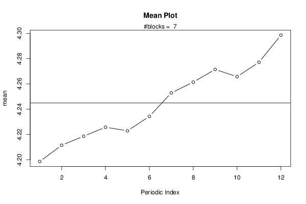
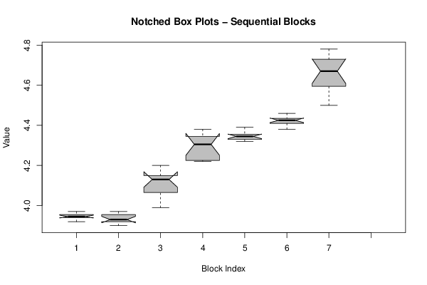
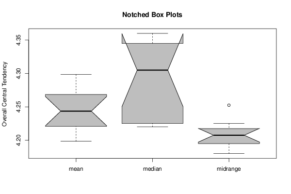
| Title produced by software | Mean Plot | ||||||||||||||||||||
| Date of computation | Wed, 16 Oct 2013 14:13:51 -0400 | ||||||||||||||||||||
| Cite this page as follows | Statistical Computations at FreeStatistics.org, Office for Research Development and Education, URL https://freestatistics.org/blog/index.php?v=date/2013/Oct/16/t1381947261rs5ly282mvt50g5.htm/, Retrieved Sat, 27 Apr 2024 22:19:04 +0000 | ||||||||||||||||||||
| Statistical Computations at FreeStatistics.org, Office for Research Development and Education, URL https://freestatistics.org/blog/index.php?pk=216250, Retrieved Sat, 27 Apr 2024 22:19:04 +0000 | |||||||||||||||||||||
| QR Codes: | |||||||||||||||||||||
|
| |||||||||||||||||||||
| Original text written by user: | |||||||||||||||||||||
| IsPrivate? | No (this computation is public) | ||||||||||||||||||||
| User-defined keywords | |||||||||||||||||||||
| Estimated Impact | 71 | ||||||||||||||||||||
Tree of Dependent Computations | |||||||||||||||||||||
| Family? (F = Feedback message, R = changed R code, M = changed R Module, P = changed Parameters, D = changed Data) | |||||||||||||||||||||
| - [Mean Plot] [] [2013-10-16 18:13:51] [12e977ea58b1a83461bd6217bf886aa8] [Current] | |||||||||||||||||||||
| Feedback Forum | |||||||||||||||||||||
Post a new message | |||||||||||||||||||||
Dataset | |||||||||||||||||||||
| Dataseries X: | |||||||||||||||||||||
3,96 3,97 3,96 3,95 3,94 3,94 3,95 3,93 3,94 3,92 3,95 3,94 3,95 3,92 3,92 3,92 3,92 3,9 3,92 3,94 3,96 3,95 3,96 3,97 3,99 4 4,05 4,08 4,09 4,12 4,14 4,15 4,15 4,15 4,15 4,2 4,22 4,22 4,22 4,23 4,3 4,29 4,32 4,31 4,35 4,34 4,35 4,38 4,39 4,38 4,34 4,33 4,33 4,33 4,33 4,32 4,35 4,35 4,35 4,36 4,38 4,41 4,43 4,42 4,43 4,43 4,42 4,46 4,44 4,41 4,41 4,46 4,5 4,58 4,61 4,65 4,55 4,63 4,69 4,72 4,71 4,74 4,77 4,78 | |||||||||||||||||||||
Tables (Output of Computation) | |||||||||||||||||||||
| |||||||||||||||||||||
Figures (Output of Computation) | |||||||||||||||||||||
Input Parameters & R Code | |||||||||||||||||||||
| Parameters (Session): | |||||||||||||||||||||
| par1 = 12 ; | |||||||||||||||||||||
| Parameters (R input): | |||||||||||||||||||||
| par1 = 12 ; | |||||||||||||||||||||
| R code (references can be found in the software module): | |||||||||||||||||||||
par1 <- as.numeric(par1) | |||||||||||||||||||||