Repository of Reproducible Computations

Free Statistics

of Irreproducible Research!

Author's title

Author

*Unverified author*

R Software Module

rwasp_autocorrelation.wasp

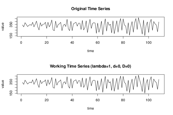
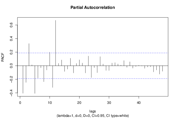
Title produced by software

(Partial) Autocorrelation Function

Date of computation

Tue, 05 Aug 2014 14:41:38 +0100

Cite this page as follows

Statistical Computations at FreeStatistics.org, Office for Research Development and Education, URL https://freestatistics.org/blog/index.php?v=date/2014/Aug/05/t1407246137kmnnrg71peai6cs.htm/, Retrieved Thu, 16 May 2024 11:52:24 +0000

Statistical Computations at FreeStatistics.org, Office for Research Development and Education, URL https://freestatistics.org/blog/index.php?pk=235409, Retrieved Thu, 16 May 2024 11:52:24 +0000

QR Codes:

Paste this QR Code to cite your computation.

Original text written by user:

IsPrivate?

No (this computation is public)

User-defined keywords

Ines Van Dessel

Estimated Impact

138

Family? (F = Feedback message, R = changed R code, M = changed R Module, P = changed Parameters, D = changed Data)

-     [Histogram] [Tijdreeks 1 - Stap 3] [2014-08-03 19:11:32] [ae3d1feb555b13e324db089723206180]
- R P   [Histogram] [Tijdreeks 1 - Stap 5] [2014-08-04 09:44:37] [74be16979710d4c4e7c6647856088456]
-   P     [Histogram] [Tijdreeks 1 - Stap 5] [2014-08-04 09:47:49] [74be16979710d4c4e7c6647856088456]
- RMP       [(Partial) Autocorrelation Function] [Tijdreeks 1 - Sta...] [2014-08-04 16:49:46] [ae3d1feb555b13e324db089723206180]
- R P         [(Partial) Autocorrelation Function] [Tijdreeks 1 - Sta...] [2014-08-05 08:15:03] [74be16979710d4c4e7c6647856088456]
- RMPD          [Harrell-Davis Quantiles] [Tijdreeks 2 - Stap 6] [2014-08-05 08:50:48] [ae3d1feb555b13e324db089723206180]
- RMP               [(Partial) Autocorrelation Function] [Tijdreeks 2 - Sta...] [2014-08-05 13:41:38] [188bf81caccb86647293be436f272d1b] [Current]
- RM                  [Variability] [Tijdreeks 2 - Sta...] [2014-08-05 14:05:00] [ae3d1feb555b13e324db089723206180] 
- RM                  [Standard Deviation-Mean Plot] [Tijdreeks 2 - Sta...] [2014-08-05 14:15:49] [ae3d1feb555b13e324db089723206180] 
- RM                  [Classical Decomposition] [Tijdreeks 2 - Sta...] [2014-08-05 14:26:32] [ae3d1feb555b13e324db089723206180] 
- RM                  [Exponential Smoothing] [Tijdreeks 2 - Sta...] [2014-08-05 14:43:00] [ae3d1feb555b13e324db089723206180] 

Feedback Forum

Post a new message

Dataseries X:

Download CSV

Histogram

Boxplots

Summary of computational transaction
Raw Input	view raw input (R code)
Raw Output	view raw output of R engine
Computing time	2 seconds
R Server	'George Udny Yule' @ yule.wessa.net

\begin{tabular}{lllllllll}
\hline
Summary of computational transaction \tabularnewline
Raw Input & view raw input (R code)  \tabularnewline
Raw Output & view raw output of R engine  \tabularnewline
Computing time & 2 seconds \tabularnewline
R Server & 'George Udny Yule' @ yule.wessa.net \tabularnewline
\hline
\end{tabular}
%Source: https://freestatistics.org/blog/index.php?pk=235409&T=0

[TABLE]
[ROW][C]Summary of computational transaction[/C][/ROW]
[ROW][C]Raw Input[/C][C]view raw input (R code) [/C][/ROW]
[ROW][C]Raw Output[/C][C]view raw output of R engine [/C][/ROW]
[ROW][C]Computing time[/C][C]2 seconds[/C][/ROW]
[ROW][C]R Server[/C][C]'George Udny Yule' @ yule.wessa.net[/C][/ROW]
[/TABLE]
Source: https://freestatistics.org/blog/index.php?pk=235409&T=0

Globally Unique Identifier (entire table): ba.freestatistics.org/blog/index.php?pk=235409&T=0

As an alternative you can also use a QR Code:

The GUIDs for individual cells are displayed in the table below:

Summary of computational transaction
Raw Input	view raw input (R code)
Raw Output	view raw output of R engine
Computing time	2 seconds
R Server	'George Udny Yule' @ yule.wessa.net

Autocorrelation Function
Time lag k	ACF(k)	T-STAT	P-value
1	-0.405261	-4.2116	2.6e-05
2	-0.040985	-0.4259	0.335504
3	0.376349	3.9111	8e-05
4	-0.279465	-2.9043	0.002232
5	-0.215105	-2.2354	0.013723
6	0.254652	2.6464	0.004675
7	-0.21244	-2.2077	0.014688
8	-0.220323	-2.2897	0.011992
9	0.324579	3.3731	0.000516
10	-0.034794	-0.3616	0.359183
11	-0.343011	-3.5647	0.000272
12	0.830334	8.6291	0
13	-0.399139	-4.148	3.4e-05
14	-0.015036	-0.1563	0.438062
15	0.35189	3.6569	0.000198
16	-0.314469	-3.2681	0.000726
17	-0.144714	-1.5039	0.067761
18	0.20565	2.1372	0.01742
19	-0.19883	-2.0663	0.020596
20	-0.132558	-1.3776	0.08559
21	0.268188	2.7871	0.003142
22	-0.056835	-0.5907	0.277994
23	-0.22042	-2.2907	0.011962
24	0.616549	6.4074	0
25	-0.377951	-3.9278	7.6e-05
26	0.011691	0.1215	0.451761
27	0.330259	3.4322	0.000425
28	-0.34806	-3.6171	0.000227
29	-0.060793	-0.6318	0.264432
30	0.160417	1.6671	0.049195
31	-0.185937	-1.9323	0.02797
32	-0.065327	-0.6789	0.249326
33	0.239998	2.4941	0.007071
34	-0.082648	-0.8589	0.196147
35	-0.096985	-1.0079	0.157878
36	0.426112	4.4283	1.1e-05
37	-0.312486	-3.2474	0.000776
38	0.011851	0.1232	0.451107
39	0.283282	2.944	0.001984
40	-0.351993	-3.658	0.000197
41	0.013326	0.1385	0.445055
42	0.104881	1.09	0.13908
43	-0.166228	-1.7275	0.043469
44	-0.025106	-0.2609	0.397328
45	0.190647	1.9813	0.025052
46	-0.106354	-1.1053	0.135751
47	-0.018537	-0.1926	0.423799
48	0.250763	2.606	0.005226

\begin{tabular}{lllllllll}
\hline
Autocorrelation Function \tabularnewline
Time lag k & ACF(k) & T-STAT & P-value \tabularnewline
1 & -0.405261 & -4.2116 & 2.6e-05 \tabularnewline
2 & -0.040985 & -0.4259 & 0.335504 \tabularnewline
3 & 0.376349 & 3.9111 & 8e-05 \tabularnewline
4 & -0.279465 & -2.9043 & 0.002232 \tabularnewline
5 & -0.215105 & -2.2354 & 0.013723 \tabularnewline
6 & 0.254652 & 2.6464 & 0.004675 \tabularnewline
7 & -0.21244 & -2.2077 & 0.014688 \tabularnewline
8 & -0.220323 & -2.2897 & 0.011992 \tabularnewline
9 & 0.324579 & 3.3731 & 0.000516 \tabularnewline
10 & -0.034794 & -0.3616 & 0.359183 \tabularnewline
11 & -0.343011 & -3.5647 & 0.000272 \tabularnewline
12 & 0.830334 & 8.6291 & 0 \tabularnewline
13 & -0.399139 & -4.148 & 3.4e-05 \tabularnewline
14 & -0.015036 & -0.1563 & 0.438062 \tabularnewline
15 & 0.35189 & 3.6569 & 0.000198 \tabularnewline
16 & -0.314469 & -3.2681 & 0.000726 \tabularnewline
17 & -0.144714 & -1.5039 & 0.067761 \tabularnewline
18 & 0.20565 & 2.1372 & 0.01742 \tabularnewline
19 & -0.19883 & -2.0663 & 0.020596 \tabularnewline
20 & -0.132558 & -1.3776 & 0.08559 \tabularnewline
21 & 0.268188 & 2.7871 & 0.003142 \tabularnewline
22 & -0.056835 & -0.5907 & 0.277994 \tabularnewline
23 & -0.22042 & -2.2907 & 0.011962 \tabularnewline
24 & 0.616549 & 6.4074 & 0 \tabularnewline
25 & -0.377951 & -3.9278 & 7.6e-05 \tabularnewline
26 & 0.011691 & 0.1215 & 0.451761 \tabularnewline
27 & 0.330259 & 3.4322 & 0.000425 \tabularnewline
28 & -0.34806 & -3.6171 & 0.000227 \tabularnewline
29 & -0.060793 & -0.6318 & 0.264432 \tabularnewline
30 & 0.160417 & 1.6671 & 0.049195 \tabularnewline
31 & -0.185937 & -1.9323 & 0.02797 \tabularnewline
32 & -0.065327 & -0.6789 & 0.249326 \tabularnewline
33 & 0.239998 & 2.4941 & 0.007071 \tabularnewline
34 & -0.082648 & -0.8589 & 0.196147 \tabularnewline
35 & -0.096985 & -1.0079 & 0.157878 \tabularnewline
36 & 0.426112 & 4.4283 & 1.1e-05 \tabularnewline
37 & -0.312486 & -3.2474 & 0.000776 \tabularnewline
38 & 0.011851 & 0.1232 & 0.451107 \tabularnewline
39 & 0.283282 & 2.944 & 0.001984 \tabularnewline
40 & -0.351993 & -3.658 & 0.000197 \tabularnewline
41 & 0.013326 & 0.1385 & 0.445055 \tabularnewline
42 & 0.104881 & 1.09 & 0.13908 \tabularnewline
43 & -0.166228 & -1.7275 & 0.043469 \tabularnewline
44 & -0.025106 & -0.2609 & 0.397328 \tabularnewline
45 & 0.190647 & 1.9813 & 0.025052 \tabularnewline
46 & -0.106354 & -1.1053 & 0.135751 \tabularnewline
47 & -0.018537 & -0.1926 & 0.423799 \tabularnewline
48 & 0.250763 & 2.606 & 0.005226 \tabularnewline
\hline
\end{tabular}
%Source: https://freestatistics.org/blog/index.php?pk=235409&T=1

[TABLE]
[ROW][C]Autocorrelation Function[/C][/ROW]
[ROW][C]Time lag k[/C][C]ACF(k)[/C][C]T-STAT[/C][C]P-value[/C][/ROW]
[ROW][C]1[/C][C]-0.405261[/C][C]-4.2116[/C][C]2.6e-05[/C][/ROW]
[ROW][C]2[/C][C]-0.040985[/C][C]-0.4259[/C][C]0.335504[/C][/ROW]
[ROW][C]3[/C][C]0.376349[/C][C]3.9111[/C][C]8e-05[/C][/ROW]
[ROW][C]4[/C][C]-0.279465[/C][C]-2.9043[/C][C]0.002232[/C][/ROW]
[ROW][C]5[/C][C]-0.215105[/C][C]-2.2354[/C][C]0.013723[/C][/ROW]
[ROW][C]6[/C][C]0.254652[/C][C]2.6464[/C][C]0.004675[/C][/ROW]
[ROW][C]7[/C][C]-0.21244[/C][C]-2.2077[/C][C]0.014688[/C][/ROW]
[ROW][C]8[/C][C]-0.220323[/C][C]-2.2897[/C][C]0.011992[/C][/ROW]
[ROW][C]9[/C][C]0.324579[/C][C]3.3731[/C][C]0.000516[/C][/ROW]
[ROW][C]10[/C][C]-0.034794[/C][C]-0.3616[/C][C]0.359183[/C][/ROW]
[ROW][C]11[/C][C]-0.343011[/C][C]-3.5647[/C][C]0.000272[/C][/ROW]
[ROW][C]12[/C][C]0.830334[/C][C]8.6291[/C][C]0[/C][/ROW]
[ROW][C]13[/C][C]-0.399139[/C][C]-4.148[/C][C]3.4e-05[/C][/ROW]
[ROW][C]14[/C][C]-0.015036[/C][C]-0.1563[/C][C]0.438062[/C][/ROW]
[ROW][C]15[/C][C]0.35189[/C][C]3.6569[/C][C]0.000198[/C][/ROW]
[ROW][C]16[/C][C]-0.314469[/C][C]-3.2681[/C][C]0.000726[/C][/ROW]
[ROW][C]17[/C][C]-0.144714[/C][C]-1.5039[/C][C]0.067761[/C][/ROW]
[ROW][C]18[/C][C]0.20565[/C][C]2.1372[/C][C]0.01742[/C][/ROW]
[ROW][C]19[/C][C]-0.19883[/C][C]-2.0663[/C][C]0.020596[/C][/ROW]
[ROW][C]20[/C][C]-0.132558[/C][C]-1.3776[/C][C]0.08559[/C][/ROW]
[ROW][C]21[/C][C]0.268188[/C][C]2.7871[/C][C]0.003142[/C][/ROW]
[ROW][C]22[/C][C]-0.056835[/C][C]-0.5907[/C][C]0.277994[/C][/ROW]
[ROW][C]23[/C][C]-0.22042[/C][C]-2.2907[/C][C]0.011962[/C][/ROW]
[ROW][C]24[/C][C]0.616549[/C][C]6.4074[/C][C]0[/C][/ROW]
[ROW][C]25[/C][C]-0.377951[/C][C]-3.9278[/C][C]7.6e-05[/C][/ROW]
[ROW][C]26[/C][C]0.011691[/C][C]0.1215[/C][C]0.451761[/C][/ROW]
[ROW][C]27[/C][C]0.330259[/C][C]3.4322[/C][C]0.000425[/C][/ROW]
[ROW][C]28[/C][C]-0.34806[/C][C]-3.6171[/C][C]0.000227[/C][/ROW]
[ROW][C]29[/C][C]-0.060793[/C][C]-0.6318[/C][C]0.264432[/C][/ROW]
[ROW][C]30[/C][C]0.160417[/C][C]1.6671[/C][C]0.049195[/C][/ROW]
[ROW][C]31[/C][C]-0.185937[/C][C]-1.9323[/C][C]0.02797[/C][/ROW]
[ROW][C]32[/C][C]-0.065327[/C][C]-0.6789[/C][C]0.249326[/C][/ROW]
[ROW][C]33[/C][C]0.239998[/C][C]2.4941[/C][C]0.007071[/C][/ROW]
[ROW][C]34[/C][C]-0.082648[/C][C]-0.8589[/C][C]0.196147[/C][/ROW]
[ROW][C]35[/C][C]-0.096985[/C][C]-1.0079[/C][C]0.157878[/C][/ROW]
[ROW][C]36[/C][C]0.426112[/C][C]4.4283[/C][C]1.1e-05[/C][/ROW]
[ROW][C]37[/C][C]-0.312486[/C][C]-3.2474[/C][C]0.000776[/C][/ROW]
[ROW][C]38[/C][C]0.011851[/C][C]0.1232[/C][C]0.451107[/C][/ROW]
[ROW][C]39[/C][C]0.283282[/C][C]2.944[/C][C]0.001984[/C][/ROW]
[ROW][C]40[/C][C]-0.351993[/C][C]-3.658[/C][C]0.000197[/C][/ROW]
[ROW][C]41[/C][C]0.013326[/C][C]0.1385[/C][C]0.445055[/C][/ROW]
[ROW][C]42[/C][C]0.104881[/C][C]1.09[/C][C]0.13908[/C][/ROW]
[ROW][C]43[/C][C]-0.166228[/C][C]-1.7275[/C][C]0.043469[/C][/ROW]
[ROW][C]44[/C][C]-0.025106[/C][C]-0.2609[/C][C]0.397328[/C][/ROW]
[ROW][C]45[/C][C]0.190647[/C][C]1.9813[/C][C]0.025052[/C][/ROW]
[ROW][C]46[/C][C]-0.106354[/C][C]-1.1053[/C][C]0.135751[/C][/ROW]
[ROW][C]47[/C][C]-0.018537[/C][C]-0.1926[/C][C]0.423799[/C][/ROW]
[ROW][C]48[/C][C]0.250763[/C][C]2.606[/C][C]0.005226[/C][/ROW]
[/TABLE]
Source: https://freestatistics.org/blog/index.php?pk=235409&T=1

Globally Unique Identifier (entire table): ba.freestatistics.org/blog/index.php?pk=235409&T=1

As an alternative you can also use a QR Code:

The GUIDs for individual cells are displayed in the table below:

Autocorrelation Function
Time lag k	ACF(k)	T-STAT	P-value
1	-0.405261	-4.2116	2.6e-05
2	-0.040985	-0.4259	0.335504
3	0.376349	3.9111	8e-05
4	-0.279465	-2.9043	0.002232
5	-0.215105	-2.2354	0.013723
6	0.254652	2.6464	0.004675
7	-0.21244	-2.2077	0.014688
8	-0.220323	-2.2897	0.011992
9	0.324579	3.3731	0.000516
10	-0.034794	-0.3616	0.359183
11	-0.343011	-3.5647	0.000272
12	0.830334	8.6291	0
13	-0.399139	-4.148	3.4e-05
14	-0.015036	-0.1563	0.438062
15	0.35189	3.6569	0.000198
16	-0.314469	-3.2681	0.000726
17	-0.144714	-1.5039	0.067761
18	0.20565	2.1372	0.01742
19	-0.19883	-2.0663	0.020596
20	-0.132558	-1.3776	0.08559
21	0.268188	2.7871	0.003142
22	-0.056835	-0.5907	0.277994
23	-0.22042	-2.2907	0.011962
24	0.616549	6.4074	0
25	-0.377951	-3.9278	7.6e-05
26	0.011691	0.1215	0.451761
27	0.330259	3.4322	0.000425
28	-0.34806	-3.6171	0.000227
29	-0.060793	-0.6318	0.264432
30	0.160417	1.6671	0.049195
31	-0.185937	-1.9323	0.02797
32	-0.065327	-0.6789	0.249326
33	0.239998	2.4941	0.007071
34	-0.082648	-0.8589	0.196147
35	-0.096985	-1.0079	0.157878
36	0.426112	4.4283	1.1e-05
37	-0.312486	-3.2474	0.000776
38	0.011851	0.1232	0.451107
39	0.283282	2.944	0.001984
40	-0.351993	-3.658	0.000197
41	0.013326	0.1385	0.445055
42	0.104881	1.09	0.13908
43	-0.166228	-1.7275	0.043469
44	-0.025106	-0.2609	0.397328
45	0.190647	1.9813	0.025052
46	-0.106354	-1.1053	0.135751
47	-0.018537	-0.1926	0.423799
48	0.250763	2.606	0.005226

Partial Autocorrelation Function
Time lag k	PACF(k)	T-STAT	P-value
1	-0.405261	-4.2116	2.6e-05
2	-0.245549	-2.5518	0.006057
3	0.32615	3.3895	0.000489
4	0.013144	0.1366	0.445802
5	-0.407595	-4.2359	2.4e-05
6	-0.180141	-1.8721	0.03195
7	-0.030533	-0.3173	0.375811
8	-0.235144	-2.4437	0.008079
9	-0.062336	-0.6478	0.259238
10	0.199176	2.0699	0.020424
11	-0.320071	-3.3263	0.000602
12	0.668893	6.9513	0
13	0.03512	0.365	0.357919
14	0.085547	0.889	0.18798
15	-0.083991	-0.8729	0.192339
16	-0.049932	-0.5189	0.302442
17	0.110215	1.1454	0.12729
18	-0.105875	-1.1003	0.136827
19	0.034373	0.3572	0.360815
20	0.087227	0.9065	0.183347
21	0.039561	0.4111	0.340895
22	-0.105699	-1.0985	0.137225
23	0.142208	1.4779	0.071177
24	-0.173835	-1.8065	0.036809
25	-0.027447	-0.2852	0.388002
26	-0.101582	-1.0557	0.146737
27	0.13443	1.397	0.082633
28	0.025246	0.2624	0.396769
29	-0.069287	-0.7201	0.236525
30	-0.070126	-0.7288	0.233858
31	0.03978	0.4134	0.340064
32	0.046131	0.4794	0.316309
33	0.02695	0.2801	0.389978
34	0.009578	0.0995	0.460449
35	0.076353	0.7935	0.214619
36	-0.023498	-0.2442	0.40377
37	0.058457	0.6075	0.272395
38	-0.03545	-0.3684	0.356647
39	-0.011253	-0.1169	0.45356
40	0.006752	0.0702	0.472096
41	-0.003815	-0.0396	0.484223
42	-0.038153	-0.3965	0.346259
43	-0.018328	-0.1905	0.424651
44	-0.016126	-0.1676	0.43361
45	-0.090729	-0.9429	0.173923
46	-0.062983	-0.6545	0.257079
47	-0.123484	-1.2833	0.10107
48	-0.081513	-0.8471	0.199404

\begin{tabular}{lllllllll}
\hline
Partial Autocorrelation Function \tabularnewline
Time lag k & PACF(k) & T-STAT & P-value \tabularnewline
1 & -0.405261 & -4.2116 & 2.6e-05 \tabularnewline
2 & -0.245549 & -2.5518 & 0.006057 \tabularnewline
3 & 0.32615 & 3.3895 & 0.000489 \tabularnewline
4 & 0.013144 & 0.1366 & 0.445802 \tabularnewline
5 & -0.407595 & -4.2359 & 2.4e-05 \tabularnewline
6 & -0.180141 & -1.8721 & 0.03195 \tabularnewline
7 & -0.030533 & -0.3173 & 0.375811 \tabularnewline
8 & -0.235144 & -2.4437 & 0.008079 \tabularnewline
9 & -0.062336 & -0.6478 & 0.259238 \tabularnewline
10 & 0.199176 & 2.0699 & 0.020424 \tabularnewline
11 & -0.320071 & -3.3263 & 0.000602 \tabularnewline
12 & 0.668893 & 6.9513 & 0 \tabularnewline
13 & 0.03512 & 0.365 & 0.357919 \tabularnewline
14 & 0.085547 & 0.889 & 0.18798 \tabularnewline
15 & -0.083991 & -0.8729 & 0.192339 \tabularnewline
16 & -0.049932 & -0.5189 & 0.302442 \tabularnewline
17 & 0.110215 & 1.1454 & 0.12729 \tabularnewline
18 & -0.105875 & -1.1003 & 0.136827 \tabularnewline
19 & 0.034373 & 0.3572 & 0.360815 \tabularnewline
20 & 0.087227 & 0.9065 & 0.183347 \tabularnewline
21 & 0.039561 & 0.4111 & 0.340895 \tabularnewline
22 & -0.105699 & -1.0985 & 0.137225 \tabularnewline
23 & 0.142208 & 1.4779 & 0.071177 \tabularnewline
24 & -0.173835 & -1.8065 & 0.036809 \tabularnewline
25 & -0.027447 & -0.2852 & 0.388002 \tabularnewline
26 & -0.101582 & -1.0557 & 0.146737 \tabularnewline
27 & 0.13443 & 1.397 & 0.082633 \tabularnewline
28 & 0.025246 & 0.2624 & 0.396769 \tabularnewline
29 & -0.069287 & -0.7201 & 0.236525 \tabularnewline
30 & -0.070126 & -0.7288 & 0.233858 \tabularnewline
31 & 0.03978 & 0.4134 & 0.340064 \tabularnewline
32 & 0.046131 & 0.4794 & 0.316309 \tabularnewline
33 & 0.02695 & 0.2801 & 0.389978 \tabularnewline
34 & 0.009578 & 0.0995 & 0.460449 \tabularnewline
35 & 0.076353 & 0.7935 & 0.214619 \tabularnewline
36 & -0.023498 & -0.2442 & 0.40377 \tabularnewline
37 & 0.058457 & 0.6075 & 0.272395 \tabularnewline
38 & -0.03545 & -0.3684 & 0.356647 \tabularnewline
39 & -0.011253 & -0.1169 & 0.45356 \tabularnewline
40 & 0.006752 & 0.0702 & 0.472096 \tabularnewline
41 & -0.003815 & -0.0396 & 0.484223 \tabularnewline
42 & -0.038153 & -0.3965 & 0.346259 \tabularnewline
43 & -0.018328 & -0.1905 & 0.424651 \tabularnewline
44 & -0.016126 & -0.1676 & 0.43361 \tabularnewline
45 & -0.090729 & -0.9429 & 0.173923 \tabularnewline
46 & -0.062983 & -0.6545 & 0.257079 \tabularnewline
47 & -0.123484 & -1.2833 & 0.10107 \tabularnewline
48 & -0.081513 & -0.8471 & 0.199404 \tabularnewline
\hline
\end{tabular}
%Source: https://freestatistics.org/blog/index.php?pk=235409&T=2

[TABLE]
[ROW][C]Partial Autocorrelation Function[/C][/ROW]
[ROW][C]Time lag k[/C][C]PACF(k)[/C][C]T-STAT[/C][C]P-value[/C][/ROW]
[ROW][C]1[/C][C]-0.405261[/C][C]-4.2116[/C][C]2.6e-05[/C][/ROW]
[ROW][C]2[/C][C]-0.245549[/C][C]-2.5518[/C][C]0.006057[/C][/ROW]
[ROW][C]3[/C][C]0.32615[/C][C]3.3895[/C][C]0.000489[/C][/ROW]
[ROW][C]4[/C][C]0.013144[/C][C]0.1366[/C][C]0.445802[/C][/ROW]
[ROW][C]5[/C][C]-0.407595[/C][C]-4.2359[/C][C]2.4e-05[/C][/ROW]
[ROW][C]6[/C][C]-0.180141[/C][C]-1.8721[/C][C]0.03195[/C][/ROW]
[ROW][C]7[/C][C]-0.030533[/C][C]-0.3173[/C][C]0.375811[/C][/ROW]
[ROW][C]8[/C][C]-0.235144[/C][C]-2.4437[/C][C]0.008079[/C][/ROW]
[ROW][C]9[/C][C]-0.062336[/C][C]-0.6478[/C][C]0.259238[/C][/ROW]
[ROW][C]10[/C][C]0.199176[/C][C]2.0699[/C][C]0.020424[/C][/ROW]
[ROW][C]11[/C][C]-0.320071[/C][C]-3.3263[/C][C]0.000602[/C][/ROW]
[ROW][C]12[/C][C]0.668893[/C][C]6.9513[/C][C]0[/C][/ROW]
[ROW][C]13[/C][C]0.03512[/C][C]0.365[/C][C]0.357919[/C][/ROW]
[ROW][C]14[/C][C]0.085547[/C][C]0.889[/C][C]0.18798[/C][/ROW]
[ROW][C]15[/C][C]-0.083991[/C][C]-0.8729[/C][C]0.192339[/C][/ROW]
[ROW][C]16[/C][C]-0.049932[/C][C]-0.5189[/C][C]0.302442[/C][/ROW]
[ROW][C]17[/C][C]0.110215[/C][C]1.1454[/C][C]0.12729[/C][/ROW]
[ROW][C]18[/C][C]-0.105875[/C][C]-1.1003[/C][C]0.136827[/C][/ROW]
[ROW][C]19[/C][C]0.034373[/C][C]0.3572[/C][C]0.360815[/C][/ROW]
[ROW][C]20[/C][C]0.087227[/C][C]0.9065[/C][C]0.183347[/C][/ROW]
[ROW][C]21[/C][C]0.039561[/C][C]0.4111[/C][C]0.340895[/C][/ROW]
[ROW][C]22[/C][C]-0.105699[/C][C]-1.0985[/C][C]0.137225[/C][/ROW]
[ROW][C]23[/C][C]0.142208[/C][C]1.4779[/C][C]0.071177[/C][/ROW]
[ROW][C]24[/C][C]-0.173835[/C][C]-1.8065[/C][C]0.036809[/C][/ROW]
[ROW][C]25[/C][C]-0.027447[/C][C]-0.2852[/C][C]0.388002[/C][/ROW]
[ROW][C]26[/C][C]-0.101582[/C][C]-1.0557[/C][C]0.146737[/C][/ROW]
[ROW][C]27[/C][C]0.13443[/C][C]1.397[/C][C]0.082633[/C][/ROW]
[ROW][C]28[/C][C]0.025246[/C][C]0.2624[/C][C]0.396769[/C][/ROW]
[ROW][C]29[/C][C]-0.069287[/C][C]-0.7201[/C][C]0.236525[/C][/ROW]
[ROW][C]30[/C][C]-0.070126[/C][C]-0.7288[/C][C]0.233858[/C][/ROW]
[ROW][C]31[/C][C]0.03978[/C][C]0.4134[/C][C]0.340064[/C][/ROW]
[ROW][C]32[/C][C]0.046131[/C][C]0.4794[/C][C]0.316309[/C][/ROW]
[ROW][C]33[/C][C]0.02695[/C][C]0.2801[/C][C]0.389978[/C][/ROW]
[ROW][C]34[/C][C]0.009578[/C][C]0.0995[/C][C]0.460449[/C][/ROW]
[ROW][C]35[/C][C]0.076353[/C][C]0.7935[/C][C]0.214619[/C][/ROW]
[ROW][C]36[/C][C]-0.023498[/C][C]-0.2442[/C][C]0.40377[/C][/ROW]
[ROW][C]37[/C][C]0.058457[/C][C]0.6075[/C][C]0.272395[/C][/ROW]
[ROW][C]38[/C][C]-0.03545[/C][C]-0.3684[/C][C]0.356647[/C][/ROW]
[ROW][C]39[/C][C]-0.011253[/C][C]-0.1169[/C][C]0.45356[/C][/ROW]
[ROW][C]40[/C][C]0.006752[/C][C]0.0702[/C][C]0.472096[/C][/ROW]
[ROW][C]41[/C][C]-0.003815[/C][C]-0.0396[/C][C]0.484223[/C][/ROW]
[ROW][C]42[/C][C]-0.038153[/C][C]-0.3965[/C][C]0.346259[/C][/ROW]
[ROW][C]43[/C][C]-0.018328[/C][C]-0.1905[/C][C]0.424651[/C][/ROW]
[ROW][C]44[/C][C]-0.016126[/C][C]-0.1676[/C][C]0.43361[/C][/ROW]
[ROW][C]45[/C][C]-0.090729[/C][C]-0.9429[/C][C]0.173923[/C][/ROW]
[ROW][C]46[/C][C]-0.062983[/C][C]-0.6545[/C][C]0.257079[/C][/ROW]
[ROW][C]47[/C][C]-0.123484[/C][C]-1.2833[/C][C]0.10107[/C][/ROW]
[ROW][C]48[/C][C]-0.081513[/C][C]-0.8471[/C][C]0.199404[/C][/ROW]
[/TABLE]
Source: https://freestatistics.org/blog/index.php?pk=235409&T=2

Globally Unique Identifier (entire table): ba.freestatistics.org/blog/index.php?pk=235409&T=2

As an alternative you can also use a QR Code:

The GUIDs for individual cells are displayed in the table below:

Partial Autocorrelation Function
Time lag k	PACF(k)	T-STAT	P-value
1	-0.405261	-4.2116	2.6e-05
2	-0.245549	-2.5518	0.006057
3	0.32615	3.3895	0.000489
4	0.013144	0.1366	0.445802
5	-0.407595	-4.2359	2.4e-05
6	-0.180141	-1.8721	0.03195
7	-0.030533	-0.3173	0.375811
8	-0.235144	-2.4437	0.008079
9	-0.062336	-0.6478	0.259238
10	0.199176	2.0699	0.020424
11	-0.320071	-3.3263	0.000602
12	0.668893	6.9513	0
13	0.03512	0.365	0.357919
14	0.085547	0.889	0.18798
15	-0.083991	-0.8729	0.192339
16	-0.049932	-0.5189	0.302442
17	0.110215	1.1454	0.12729
18	-0.105875	-1.1003	0.136827
19	0.034373	0.3572	0.360815
20	0.087227	0.9065	0.183347
21	0.039561	0.4111	0.340895
22	-0.105699	-1.0985	0.137225
23	0.142208	1.4779	0.071177
24	-0.173835	-1.8065	0.036809
25	-0.027447	-0.2852	0.388002
26	-0.101582	-1.0557	0.146737
27	0.13443	1.397	0.082633
28	0.025246	0.2624	0.396769
29	-0.069287	-0.7201	0.236525
30	-0.070126	-0.7288	0.233858
31	0.03978	0.4134	0.340064
32	0.046131	0.4794	0.316309
33	0.02695	0.2801	0.389978
34	0.009578	0.0995	0.460449
35	0.076353	0.7935	0.214619
36	-0.023498	-0.2442	0.40377
37	0.058457	0.6075	0.272395
38	-0.03545	-0.3684	0.356647
39	-0.011253	-0.1169	0.45356
40	0.006752	0.0702	0.472096
41	-0.003815	-0.0396	0.484223
42	-0.038153	-0.3965	0.346259
43	-0.018328	-0.1905	0.424651
44	-0.016126	-0.1676	0.43361
45	-0.090729	-0.9429	0.173923
46	-0.062983	-0.6545	0.257079
47	-0.123484	-1.2833	0.10107
48	-0.081513	-0.8471	0.199404

Figure 1

PNG link

Postscript link

PDF link

Figure 2

PNG link

Postscript link

PDF link

Figure 3

PNG link

Postscript link

PDF link

Parameters (Session):

Parameters (R input):

par1 = 48 ; par2 = 1 ; par3 = 0 ; par4 = 0 ; par5 = 12 ; par6 = White Noise ; par7 = 0.95 ; par8 = ;

R code (references can be found in the software module):

if (par1 == 'Default') {
par1 = 10*log10(length(x))
} else {
par1 <- as.numeric(par1)
}
par2 <- as.numeric(par2)
par3 <- as.numeric(par3)
par4 <- as.numeric(par4)
par5 <- as.numeric(par5)
if (par6 == 'White Noise') par6 <- 'white' else par6 <- 'ma'
par7 <- as.numeric(par7)
if (par8 != '') par8 <- as.numeric(par8)
ox <- x
if (par8 == '') {
if (par2 == 0) {
x <- log(x)
} else {
x <- (x ^ par2 - 1) / par2
}
} else {
x <- log(x,base=par8)
}
if (par3 > 0) x <- diff(x,lag=1,difference=par3)
if (par4 > 0) x <- diff(x,lag=par5,difference=par4)
bitmap(file='picts.png')
op <- par(mfrow=c(2,1))
plot(ox,type='l',main='Original Time Series',xlab='time',ylab='value')
if (par8=='') {
mytitle <- paste('Working Time Series (lambda=',par2,', d=',par3,', D=',par4,')',sep='')
mysub <- paste('(lambda=',par2,', d=',par3,', D=',par4,', CI=', par7, ', CI type=',par6,')',sep='')
} else {
mytitle <- paste('Working Time Series (base=',par8,', d=',par3,', D=',par4,')',sep='')
mysub <- paste('(base=',par8,', d=',par3,', D=',par4,', CI=', par7, ', CI type=',par6,')',sep='')
}
plot(x,type='l', main=mytitle,xlab='time',ylab='value')
par(op)
dev.off()
bitmap(file='pic1.png')
racf <- acf(x, par1, main='Autocorrelation', xlab='time lag', ylab='ACF', ci.type=par6, ci=par7, sub=mysub)
dev.off()
bitmap(file='pic2.png')
rpacf <- pacf(x,par1,main='Partial Autocorrelation',xlab='lags',ylab='PACF',sub=mysub)
dev.off()
(myacf <- c(racf$acf))
(mypacf <- c(rpacf$acf))
lengthx <- length(x)
sqrtn <- sqrt(lengthx)
load(file='createtable')
a<-table.start()
a<-table.row.start(a)
a<-table.element(a,'Autocorrelation Function',4,TRUE)
a<-table.row.end(a)
a<-table.row.start(a)
a<-table.element(a,'Time lag k',header=TRUE)
a<-table.element(a,hyperlink('basics.htm','ACF(k)','click here for more information about the Autocorrelation Function'),header=TRUE)
a<-table.element(a,'T-STAT',header=TRUE)
a<-table.element(a,'P-value',header=TRUE)
a<-table.row.end(a)
for (i in 2:(par1+1)) {
a<-table.row.start(a)
a<-table.element(a,i-1,header=TRUE)
a<-table.element(a,round(myacf[i],6))
mytstat <- myacf[i]*sqrtn
a<-table.element(a,round(mytstat,4))
a<-table.element(a,round(1-pt(abs(mytstat),lengthx),6))
a<-table.row.end(a)
}
a<-table.end(a)
table.save(a,file='mytable.tab')
a<-table.start()
a<-table.row.start(a)
a<-table.element(a,'Partial Autocorrelation Function',4,TRUE)
a<-table.row.end(a)
a<-table.row.start(a)
a<-table.element(a,'Time lag k',header=TRUE)
a<-table.element(a,hyperlink('basics.htm','PACF(k)','click here for more information about the Partial Autocorrelation Function'),header=TRUE)
a<-table.element(a,'T-STAT',header=TRUE)
a<-table.element(a,'P-value',header=TRUE)
a<-table.row.end(a)
for (i in 1:par1) {
a<-table.row.start(a)
a<-table.element(a,i,header=TRUE)
a<-table.element(a,round(mypacf[i],6))
mytstat <- mypacf[i]*sqrtn
a<-table.element(a,round(mytstat,4))
a<-table.element(a,round(1-pt(abs(mytstat),lengthx),6))
a<-table.row.end(a)
}
a<-table.end(a)
table.save(a,file='mytable1.tab')

Free Statistics

Description of Statistical Computation

Tree of Dependent Computations

Dataset

Tables (Output of Computation)

Figures (Output of Computation)

Input Parameters & R Code