Free Statistics
of Irreproducible Research!
Description of Statistical Computation | |||||||||||||||||||||
|---|---|---|---|---|---|---|---|---|---|---|---|---|---|---|---|---|---|---|---|---|---|
| Author's title | |||||||||||||||||||||
| Author | *Unverified author* | ||||||||||||||||||||
| R Software Module | rwasp_meanplot.wasp | ||||||||||||||||||||
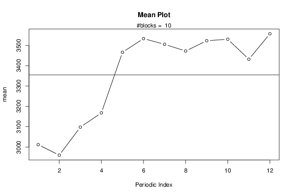
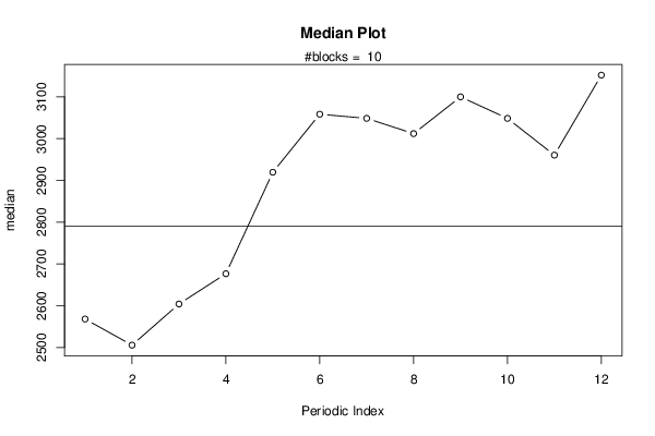
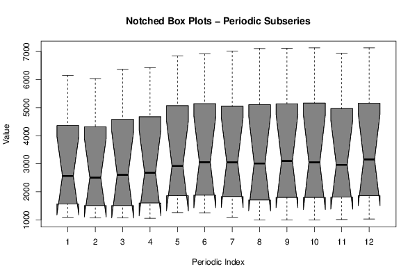
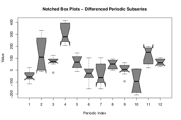
| Title produced by software | Mean Plot | ||||||||||||||||||||
| Date of computation | Sun, 17 Aug 2014 18:27:46 +0100 | ||||||||||||||||||||
| Cite this page as follows | Statistical Computations at FreeStatistics.org, Office for Research Development and Education, URL https://freestatistics.org/blog/index.php?v=date/2014/Aug/17/t14082965368u1tjjfy0meq58y.htm/, Retrieved Thu, 16 May 2024 18:20:38 +0000 | ||||||||||||||||||||
| Statistical Computations at FreeStatistics.org, Office for Research Development and Education, URL https://freestatistics.org/blog/index.php?pk=235627, Retrieved Thu, 16 May 2024 18:20:38 +0000 | |||||||||||||||||||||
| QR Codes: | |||||||||||||||||||||
|
| |||||||||||||||||||||
| Original text written by user: | |||||||||||||||||||||
| IsPrivate? | No (this computation is public) | ||||||||||||||||||||
| User-defined keywords | Van Reusel Raphael | ||||||||||||||||||||
| Estimated Impact | 101 | ||||||||||||||||||||
Tree of Dependent Computations | |||||||||||||||||||||
| Family? (F = Feedback message, R = changed R code, M = changed R Module, P = changed Parameters, D = changed Data) | |||||||||||||||||||||
| - [Harrell-Davis Quantiles] [Tijdreeks 1] [2014-08-17 17:04:09] [01050b0485b0192e33ca8050be87927f] - RMP [Mean Plot] [Tijdreeks 1] [2014-08-17 17:27:46] [bf566d88435d8cc6ce5d208f6f8dd684] [Current] | |||||||||||||||||||||
| Feedback Forum | |||||||||||||||||||||
Post a new message | |||||||||||||||||||||
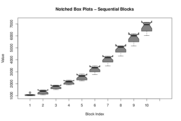
Dataset | |||||||||||||||||||||
| Dataseries X: | |||||||||||||||||||||
1095 1085 1075 1054 1261 1250 1095 992 1002 1002 1013 1033 1095 1075 1106 1157 1447 1447 1385 1323 1374 1436 1447 1478 1571 1509 1509 1602 1860 1881 1829 1705 1798 1798 1808 1860 1901 1922 1922 1984 2222 2284 2294 2139 2222 2191 2129 2263 2294 2242 2253 2325 2594 2728 2728 2666 2759 2666 2614 2811 2842 2769 2955 3028 3245 3389 3369 3358 3441 3431 3307 3493 3555 3493 3751 3875 4164 4278 4247 4185 4237 4299 4092 4257 4361 4319 4588 4681 5074 5146 5053 5105 5136 5167 4970 5156 5259 5156 5456 5549 5952 6014 6034 6138 6138 6179 5993 6086 6148 6034 6365 6427 6840 6913 7016 7109 7119 7130 6944 7130 | |||||||||||||||||||||
Tables (Output of Computation) | |||||||||||||||||||||
| |||||||||||||||||||||
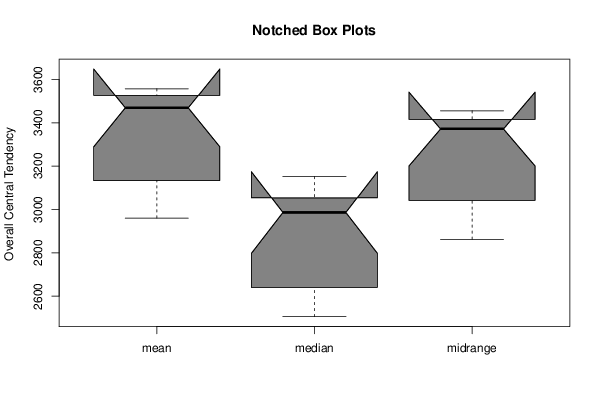
Figures (Output of Computation) | |||||||||||||||||||||
Input Parameters & R Code | |||||||||||||||||||||
| Parameters (Session): | |||||||||||||||||||||
| par1 = 12 ; | |||||||||||||||||||||
| Parameters (R input): | |||||||||||||||||||||
| par1 = 12 ; | |||||||||||||||||||||
| R code (references can be found in the software module): | |||||||||||||||||||||
par1 <- as.numeric(par1) | |||||||||||||||||||||