Repository of Reproducible Computations

Free Statistics

of Irreproducible Research!

Author's title

Author

*Unverified author*

R Software Module

rwasp_decompose.wasp

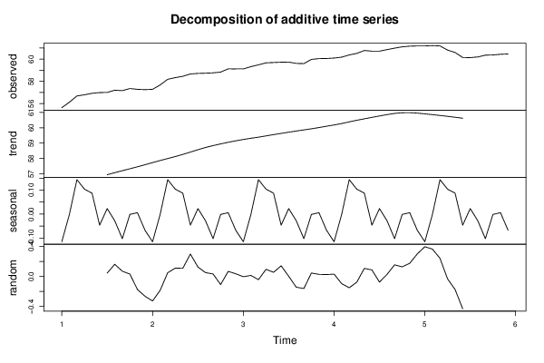
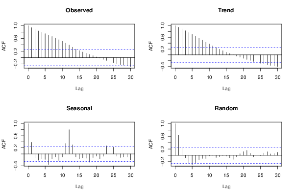
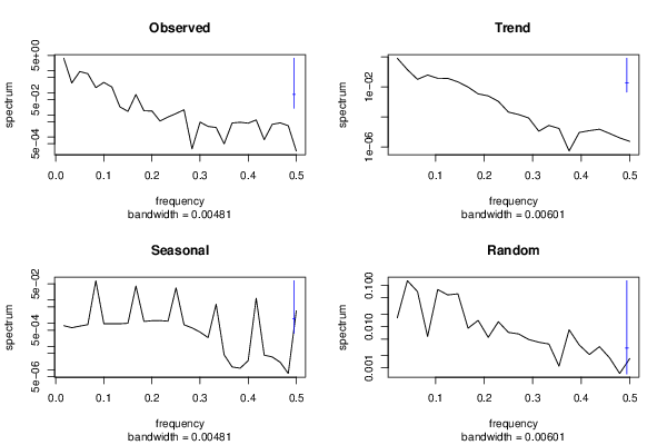
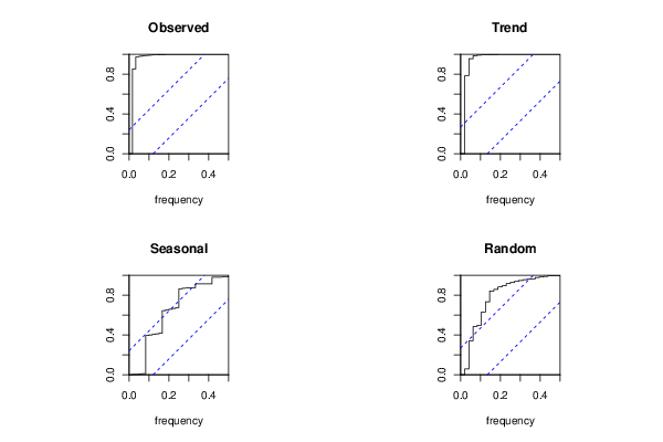
Title produced by software

Classical Decomposition

Date of computation

Mon, 12 May 2014 13:59:56 -0400

Cite this page as follows

Statistical Computations at FreeStatistics.org, Office for Research Development and Education, URL https://freestatistics.org/blog/index.php?v=date/2014/May/12/t1399917752ply1con6d3hjof6.htm/, Retrieved Wed, 15 May 2024 02:14:21 +0000

Statistical Computations at FreeStatistics.org, Office for Research Development and Education, URL https://freestatistics.org/blog/index.php?pk=234841, Retrieved Wed, 15 May 2024 02:14:21 +0000

QR Codes:

Paste this QR Code to cite your computation.

Original text written by user:

IsPrivate?

No (this computation is public)

User-defined keywords

Estimated Impact

117

Family? (F = Feedback message, R = changed R code, M = changed R Module, P = changed Parameters, D = changed Data)

-       [Classical Decomposition] [] [2014-05-12 17:59:56] [3ace99d75142efe6ae27f9378c84deb8] [Current]

Feedback Forum

Post a new message

Dataseries X:

Download CSV

Histogram

Boxplots

Summary of computational transaction
Raw Input	view raw input (R code)
Raw Output	view raw output of R engine
Computing time	3 seconds
R Server	'Herman Ole Andreas Wold' @ wold.wessa.net

\begin{tabular}{lllllllll}
\hline
Summary of computational transaction \tabularnewline
Raw Input & view raw input (R code)  \tabularnewline
Raw Output & view raw output of R engine  \tabularnewline
Computing time & 3 seconds \tabularnewline
R Server & 'Herman Ole Andreas Wold' @ wold.wessa.net \tabularnewline
\hline
\end{tabular}
%Source: https://freestatistics.org/blog/index.php?pk=234841&T=0

[TABLE]
[ROW][C]Summary of computational transaction[/C][/ROW]
[ROW][C]Raw Input[/C][C]view raw input (R code) [/C][/ROW]
[ROW][C]Raw Output[/C][C]view raw output of R engine [/C][/ROW]
[ROW][C]Computing time[/C][C]3 seconds[/C][/ROW]
[ROW][C]R Server[/C][C]'Herman Ole Andreas Wold' @ wold.wessa.net[/C][/ROW]
[/TABLE]
Source: https://freestatistics.org/blog/index.php?pk=234841&T=0

Globally Unique Identifier (entire table): ba.freestatistics.org/blog/index.php?pk=234841&T=0

As an alternative you can also use a QR Code:

The GUIDs for individual cells are displayed in the table below:

Summary of computational transaction
Raw Input	view raw input (R code)
Raw Output	view raw output of R engine
Computing time	3 seconds
R Server	'Herman Ole Andreas Wold' @ wold.wessa.net

Classical Decomposition by Moving Averages
t	Observations	Fit	Trend	Seasonal	Random
1	55.64	NA	NA	-0.115616	NA
2	56.13	NA	NA	-0.00186632	NA
3	56.69	NA	NA	0.143759	NA
4	56.8	NA	NA	0.104071	NA
5	56.93	NA	NA	0.0873003	NA
6	57	NA	NA	-0.0464497	NA
7	57.01	56.9658	56.9429	0.0229253	0.044158
8	57.21	57.0483	57.0762	-0.027908	0.161658
9	57.17	57.1005	57.2033	-0.102804	0.0694705
10	57.36	57.3284	57.33	-0.00155382	0.0315538
11	57.29	57.4638	57.4579	0.00584201	-0.173759
12	57.26	57.5236	57.5912	-0.0676997	-0.26355
13	57.29	57.6165	57.7321	-0.115616	-0.326467
14	57.68	57.8652	57.8671	-0.00186632	-0.185217
15	58.19	58.1413	57.9975	0.143759	0.0487413
16	58.34	58.2299	58.1258	0.104071	0.110095
17	58.46	58.3515	58.2642	0.0873003	0.108533
18	58.67	58.3719	58.4183	-0.0464497	0.298116
19	58.72	58.595	58.5721	0.0229253	0.124991
20	58.74	58.6892	58.7171	-0.027908	0.0508247
21	58.77	58.7372	58.84	-0.102804	0.0328038
22	58.84	58.948	58.9496	-0.00155382	-0.10803
23	59.13	59.0625	59.0567	0.00584201	0.0674913
24	59.12	59.0848	59.1525	-0.0676997	0.0351997
25	59.12	59.1236	59.2392	-0.115616	-0.00355035
26	59.33	59.3165	59.3183	-0.00186632	0.013533
27	59.49	59.5333	59.3896	0.143759	-0.043342
28	59.67	59.5757	59.4717	0.104071	0.0942622
29	59.7	59.6448	59.5575	0.0873003	0.0551997
30	59.73	59.5886	59.635	-0.0464497	0.14145
31	59.74	59.7379	59.715	0.0229253	0.00207465
32	59.62	59.7633	59.7912	-0.027908	-0.143342
33	59.6	59.7609	59.8637	-0.102804	-0.160946
34	59.98	59.9347	59.9362	-0.00155382	0.0453038
35	60.05	60.0225	60.0167	0.00584201	0.0274913
36	60.06	60.0352	60.1029	-0.0676997	0.024783
37	60.1	60.0694	60.185	-0.115616	0.0306163
38	60.18	60.2756	60.2775	-0.00186632	-0.0956337
39	60.38	60.5308	60.3871	0.143759	-0.150842
40	60.52	60.5962	60.4921	0.104071	-0.0761545
41	60.78	60.6731	60.5858	0.0873003	0.106866
42	60.72	60.6331	60.6796	-0.0464497	0.0868663
43	60.72	60.795	60.7721	0.0229253	-0.0750087
44	60.86	60.8329	60.8608	-0.027908	0.0270747
45	60.99	60.8351	60.9379	-0.102804	0.154887
46	61.11	60.9826	60.9842	-0.00155382	0.127387
47	61.17	60.995	60.9892	0.00584201	0.174991
48	61.19	60.8902	60.9579	-0.0676997	0.299783
49	61.19	60.7944	60.91	-0.115616	0.395616
50	61.22	60.8565	60.8583	-0.00186632	0.363533
51	61.19	60.9483	60.8046	0.143759	0.241658
52	60.82	60.852	60.7479	0.104071	-0.0319878
53	60.6	60.7744	60.6871	0.0873003	-0.174384
54	60.15	60.5802	60.6267	-0.0464497	-0.430217
55	60.14	NA	NA	0.0229253	NA
56	60.2	NA	NA	-0.027908	NA
57	60.36	NA	NA	-0.102804	NA
58	60.38	NA	NA	-0.00155382	NA
59	60.44	NA	NA	0.00584201	NA
60	60.47	NA	NA	-0.0676997	NA

\begin{tabular}{lllllllll}
\hline
Classical Decomposition by Moving Averages \tabularnewline
t & Observations & Fit & Trend & Seasonal & Random \tabularnewline
1 & 55.64 & NA & NA & -0.115616 & NA \tabularnewline
2 & 56.13 & NA & NA & -0.00186632 & NA \tabularnewline
3 & 56.69 & NA & NA & 0.143759 & NA \tabularnewline
4 & 56.8 & NA & NA & 0.104071 & NA \tabularnewline
5 & 56.93 & NA & NA & 0.0873003 & NA \tabularnewline
6 & 57 & NA & NA & -0.0464497 & NA \tabularnewline
7 & 57.01 & 56.9658 & 56.9429 & 0.0229253 & 0.044158 \tabularnewline
8 & 57.21 & 57.0483 & 57.0762 & -0.027908 & 0.161658 \tabularnewline
9 & 57.17 & 57.1005 & 57.2033 & -0.102804 & 0.0694705 \tabularnewline
10 & 57.36 & 57.3284 & 57.33 & -0.00155382 & 0.0315538 \tabularnewline
11 & 57.29 & 57.4638 & 57.4579 & 0.00584201 & -0.173759 \tabularnewline
12 & 57.26 & 57.5236 & 57.5912 & -0.0676997 & -0.26355 \tabularnewline
13 & 57.29 & 57.6165 & 57.7321 & -0.115616 & -0.326467 \tabularnewline
14 & 57.68 & 57.8652 & 57.8671 & -0.00186632 & -0.185217 \tabularnewline
15 & 58.19 & 58.1413 & 57.9975 & 0.143759 & 0.0487413 \tabularnewline
16 & 58.34 & 58.2299 & 58.1258 & 0.104071 & 0.110095 \tabularnewline
17 & 58.46 & 58.3515 & 58.2642 & 0.0873003 & 0.108533 \tabularnewline
18 & 58.67 & 58.3719 & 58.4183 & -0.0464497 & 0.298116 \tabularnewline
19 & 58.72 & 58.595 & 58.5721 & 0.0229253 & 0.124991 \tabularnewline
20 & 58.74 & 58.6892 & 58.7171 & -0.027908 & 0.0508247 \tabularnewline
21 & 58.77 & 58.7372 & 58.84 & -0.102804 & 0.0328038 \tabularnewline
22 & 58.84 & 58.948 & 58.9496 & -0.00155382 & -0.10803 \tabularnewline
23 & 59.13 & 59.0625 & 59.0567 & 0.00584201 & 0.0674913 \tabularnewline
24 & 59.12 & 59.0848 & 59.1525 & -0.0676997 & 0.0351997 \tabularnewline
25 & 59.12 & 59.1236 & 59.2392 & -0.115616 & -0.00355035 \tabularnewline
26 & 59.33 & 59.3165 & 59.3183 & -0.00186632 & 0.013533 \tabularnewline
27 & 59.49 & 59.5333 & 59.3896 & 0.143759 & -0.043342 \tabularnewline
28 & 59.67 & 59.5757 & 59.4717 & 0.104071 & 0.0942622 \tabularnewline
29 & 59.7 & 59.6448 & 59.5575 & 0.0873003 & 0.0551997 \tabularnewline
30 & 59.73 & 59.5886 & 59.635 & -0.0464497 & 0.14145 \tabularnewline
31 & 59.74 & 59.7379 & 59.715 & 0.0229253 & 0.00207465 \tabularnewline
32 & 59.62 & 59.7633 & 59.7912 & -0.027908 & -0.143342 \tabularnewline
33 & 59.6 & 59.7609 & 59.8637 & -0.102804 & -0.160946 \tabularnewline
34 & 59.98 & 59.9347 & 59.9362 & -0.00155382 & 0.0453038 \tabularnewline
35 & 60.05 & 60.0225 & 60.0167 & 0.00584201 & 0.0274913 \tabularnewline
36 & 60.06 & 60.0352 & 60.1029 & -0.0676997 & 0.024783 \tabularnewline
37 & 60.1 & 60.0694 & 60.185 & -0.115616 & 0.0306163 \tabularnewline
38 & 60.18 & 60.2756 & 60.2775 & -0.00186632 & -0.0956337 \tabularnewline
39 & 60.38 & 60.5308 & 60.3871 & 0.143759 & -0.150842 \tabularnewline
40 & 60.52 & 60.5962 & 60.4921 & 0.104071 & -0.0761545 \tabularnewline
41 & 60.78 & 60.6731 & 60.5858 & 0.0873003 & 0.106866 \tabularnewline
42 & 60.72 & 60.6331 & 60.6796 & -0.0464497 & 0.0868663 \tabularnewline
43 & 60.72 & 60.795 & 60.7721 & 0.0229253 & -0.0750087 \tabularnewline
44 & 60.86 & 60.8329 & 60.8608 & -0.027908 & 0.0270747 \tabularnewline
45 & 60.99 & 60.8351 & 60.9379 & -0.102804 & 0.154887 \tabularnewline
46 & 61.11 & 60.9826 & 60.9842 & -0.00155382 & 0.127387 \tabularnewline
47 & 61.17 & 60.995 & 60.9892 & 0.00584201 & 0.174991 \tabularnewline
48 & 61.19 & 60.8902 & 60.9579 & -0.0676997 & 0.299783 \tabularnewline
49 & 61.19 & 60.7944 & 60.91 & -0.115616 & 0.395616 \tabularnewline
50 & 61.22 & 60.8565 & 60.8583 & -0.00186632 & 0.363533 \tabularnewline
51 & 61.19 & 60.9483 & 60.8046 & 0.143759 & 0.241658 \tabularnewline
52 & 60.82 & 60.852 & 60.7479 & 0.104071 & -0.0319878 \tabularnewline
53 & 60.6 & 60.7744 & 60.6871 & 0.0873003 & -0.174384 \tabularnewline
54 & 60.15 & 60.5802 & 60.6267 & -0.0464497 & -0.430217 \tabularnewline
55 & 60.14 & NA & NA & 0.0229253 & NA \tabularnewline
56 & 60.2 & NA & NA & -0.027908 & NA \tabularnewline
57 & 60.36 & NA & NA & -0.102804 & NA \tabularnewline
58 & 60.38 & NA & NA & -0.00155382 & NA \tabularnewline
59 & 60.44 & NA & NA & 0.00584201 & NA \tabularnewline
60 & 60.47 & NA & NA & -0.0676997 & NA \tabularnewline
\hline
\end{tabular}
%Source: https://freestatistics.org/blog/index.php?pk=234841&T=1

[TABLE]
[ROW][C]Classical Decomposition by Moving Averages[/C][/ROW]
[ROW][C]t[/C][C]Observations[/C][C]Fit[/C][C]Trend[/C][C]Seasonal[/C][C]Random[/C][/ROW]
[ROW][C]1[/C][C]55.64[/C][C]NA[/C][C]NA[/C][C]-0.115616[/C][C]NA[/C][/ROW]
[ROW][C]2[/C][C]56.13[/C][C]NA[/C][C]NA[/C][C]-0.00186632[/C][C]NA[/C][/ROW]
[ROW][C]3[/C][C]56.69[/C][C]NA[/C][C]NA[/C][C]0.143759[/C][C]NA[/C][/ROW]
[ROW][C]4[/C][C]56.8[/C][C]NA[/C][C]NA[/C][C]0.104071[/C][C]NA[/C][/ROW]
[ROW][C]5[/C][C]56.93[/C][C]NA[/C][C]NA[/C][C]0.0873003[/C][C]NA[/C][/ROW]
[ROW][C]6[/C][C]57[/C][C]NA[/C][C]NA[/C][C]-0.0464497[/C][C]NA[/C][/ROW]
[ROW][C]7[/C][C]57.01[/C][C]56.9658[/C][C]56.9429[/C][C]0.0229253[/C][C]0.044158[/C][/ROW]
[ROW][C]8[/C][C]57.21[/C][C]57.0483[/C][C]57.0762[/C][C]-0.027908[/C][C]0.161658[/C][/ROW]
[ROW][C]9[/C][C]57.17[/C][C]57.1005[/C][C]57.2033[/C][C]-0.102804[/C][C]0.0694705[/C][/ROW]
[ROW][C]10[/C][C]57.36[/C][C]57.3284[/C][C]57.33[/C][C]-0.00155382[/C][C]0.0315538[/C][/ROW]
[ROW][C]11[/C][C]57.29[/C][C]57.4638[/C][C]57.4579[/C][C]0.00584201[/C][C]-0.173759[/C][/ROW]
[ROW][C]12[/C][C]57.26[/C][C]57.5236[/C][C]57.5912[/C][C]-0.0676997[/C][C]-0.26355[/C][/ROW]
[ROW][C]13[/C][C]57.29[/C][C]57.6165[/C][C]57.7321[/C][C]-0.115616[/C][C]-0.326467[/C][/ROW]
[ROW][C]14[/C][C]57.68[/C][C]57.8652[/C][C]57.8671[/C][C]-0.00186632[/C][C]-0.185217[/C][/ROW]
[ROW][C]15[/C][C]58.19[/C][C]58.1413[/C][C]57.9975[/C][C]0.143759[/C][C]0.0487413[/C][/ROW]
[ROW][C]16[/C][C]58.34[/C][C]58.2299[/C][C]58.1258[/C][C]0.104071[/C][C]0.110095[/C][/ROW]
[ROW][C]17[/C][C]58.46[/C][C]58.3515[/C][C]58.2642[/C][C]0.0873003[/C][C]0.108533[/C][/ROW]
[ROW][C]18[/C][C]58.67[/C][C]58.3719[/C][C]58.4183[/C][C]-0.0464497[/C][C]0.298116[/C][/ROW]
[ROW][C]19[/C][C]58.72[/C][C]58.595[/C][C]58.5721[/C][C]0.0229253[/C][C]0.124991[/C][/ROW]
[ROW][C]20[/C][C]58.74[/C][C]58.6892[/C][C]58.7171[/C][C]-0.027908[/C][C]0.0508247[/C][/ROW]
[ROW][C]21[/C][C]58.77[/C][C]58.7372[/C][C]58.84[/C][C]-0.102804[/C][C]0.0328038[/C][/ROW]
[ROW][C]22[/C][C]58.84[/C][C]58.948[/C][C]58.9496[/C][C]-0.00155382[/C][C]-0.10803[/C][/ROW]
[ROW][C]23[/C][C]59.13[/C][C]59.0625[/C][C]59.0567[/C][C]0.00584201[/C][C]0.0674913[/C][/ROW]
[ROW][C]24[/C][C]59.12[/C][C]59.0848[/C][C]59.1525[/C][C]-0.0676997[/C][C]0.0351997[/C][/ROW]
[ROW][C]25[/C][C]59.12[/C][C]59.1236[/C][C]59.2392[/C][C]-0.115616[/C][C]-0.00355035[/C][/ROW]
[ROW][C]26[/C][C]59.33[/C][C]59.3165[/C][C]59.3183[/C][C]-0.00186632[/C][C]0.013533[/C][/ROW]
[ROW][C]27[/C][C]59.49[/C][C]59.5333[/C][C]59.3896[/C][C]0.143759[/C][C]-0.043342[/C][/ROW]
[ROW][C]28[/C][C]59.67[/C][C]59.5757[/C][C]59.4717[/C][C]0.104071[/C][C]0.0942622[/C][/ROW]
[ROW][C]29[/C][C]59.7[/C][C]59.6448[/C][C]59.5575[/C][C]0.0873003[/C][C]0.0551997[/C][/ROW]
[ROW][C]30[/C][C]59.73[/C][C]59.5886[/C][C]59.635[/C][C]-0.0464497[/C][C]0.14145[/C][/ROW]
[ROW][C]31[/C][C]59.74[/C][C]59.7379[/C][C]59.715[/C][C]0.0229253[/C][C]0.00207465[/C][/ROW]
[ROW][C]32[/C][C]59.62[/C][C]59.7633[/C][C]59.7912[/C][C]-0.027908[/C][C]-0.143342[/C][/ROW]
[ROW][C]33[/C][C]59.6[/C][C]59.7609[/C][C]59.8637[/C][C]-0.102804[/C][C]-0.160946[/C][/ROW]
[ROW][C]34[/C][C]59.98[/C][C]59.9347[/C][C]59.9362[/C][C]-0.00155382[/C][C]0.0453038[/C][/ROW]
[ROW][C]35[/C][C]60.05[/C][C]60.0225[/C][C]60.0167[/C][C]0.00584201[/C][C]0.0274913[/C][/ROW]
[ROW][C]36[/C][C]60.06[/C][C]60.0352[/C][C]60.1029[/C][C]-0.0676997[/C][C]0.024783[/C][/ROW]
[ROW][C]37[/C][C]60.1[/C][C]60.0694[/C][C]60.185[/C][C]-0.115616[/C][C]0.0306163[/C][/ROW]
[ROW][C]38[/C][C]60.18[/C][C]60.2756[/C][C]60.2775[/C][C]-0.00186632[/C][C]-0.0956337[/C][/ROW]
[ROW][C]39[/C][C]60.38[/C][C]60.5308[/C][C]60.3871[/C][C]0.143759[/C][C]-0.150842[/C][/ROW]
[ROW][C]40[/C][C]60.52[/C][C]60.5962[/C][C]60.4921[/C][C]0.104071[/C][C]-0.0761545[/C][/ROW]
[ROW][C]41[/C][C]60.78[/C][C]60.6731[/C][C]60.5858[/C][C]0.0873003[/C][C]0.106866[/C][/ROW]
[ROW][C]42[/C][C]60.72[/C][C]60.6331[/C][C]60.6796[/C][C]-0.0464497[/C][C]0.0868663[/C][/ROW]
[ROW][C]43[/C][C]60.72[/C][C]60.795[/C][C]60.7721[/C][C]0.0229253[/C][C]-0.0750087[/C][/ROW]
[ROW][C]44[/C][C]60.86[/C][C]60.8329[/C][C]60.8608[/C][C]-0.027908[/C][C]0.0270747[/C][/ROW]
[ROW][C]45[/C][C]60.99[/C][C]60.8351[/C][C]60.9379[/C][C]-0.102804[/C][C]0.154887[/C][/ROW]
[ROW][C]46[/C][C]61.11[/C][C]60.9826[/C][C]60.9842[/C][C]-0.00155382[/C][C]0.127387[/C][/ROW]
[ROW][C]47[/C][C]61.17[/C][C]60.995[/C][C]60.9892[/C][C]0.00584201[/C][C]0.174991[/C][/ROW]
[ROW][C]48[/C][C]61.19[/C][C]60.8902[/C][C]60.9579[/C][C]-0.0676997[/C][C]0.299783[/C][/ROW]
[ROW][C]49[/C][C]61.19[/C][C]60.7944[/C][C]60.91[/C][C]-0.115616[/C][C]0.395616[/C][/ROW]
[ROW][C]50[/C][C]61.22[/C][C]60.8565[/C][C]60.8583[/C][C]-0.00186632[/C][C]0.363533[/C][/ROW]
[ROW][C]51[/C][C]61.19[/C][C]60.9483[/C][C]60.8046[/C][C]0.143759[/C][C]0.241658[/C][/ROW]
[ROW][C]52[/C][C]60.82[/C][C]60.852[/C][C]60.7479[/C][C]0.104071[/C][C]-0.0319878[/C][/ROW]
[ROW][C]53[/C][C]60.6[/C][C]60.7744[/C][C]60.6871[/C][C]0.0873003[/C][C]-0.174384[/C][/ROW]
[ROW][C]54[/C][C]60.15[/C][C]60.5802[/C][C]60.6267[/C][C]-0.0464497[/C][C]-0.430217[/C][/ROW]
[ROW][C]55[/C][C]60.14[/C][C]NA[/C][C]NA[/C][C]0.0229253[/C][C]NA[/C][/ROW]
[ROW][C]56[/C][C]60.2[/C][C]NA[/C][C]NA[/C][C]-0.027908[/C][C]NA[/C][/ROW]
[ROW][C]57[/C][C]60.36[/C][C]NA[/C][C]NA[/C][C]-0.102804[/C][C]NA[/C][/ROW]
[ROW][C]58[/C][C]60.38[/C][C]NA[/C][C]NA[/C][C]-0.00155382[/C][C]NA[/C][/ROW]
[ROW][C]59[/C][C]60.44[/C][C]NA[/C][C]NA[/C][C]0.00584201[/C][C]NA[/C][/ROW]
[ROW][C]60[/C][C]60.47[/C][C]NA[/C][C]NA[/C][C]-0.0676997[/C][C]NA[/C][/ROW]
[/TABLE]
Source: https://freestatistics.org/blog/index.php?pk=234841&T=1

Globally Unique Identifier (entire table): ba.freestatistics.org/blog/index.php?pk=234841&T=1

As an alternative you can also use a QR Code:

The GUIDs for individual cells are displayed in the table below:

Classical Decomposition by Moving Averages
t	Observations	Fit	Trend	Seasonal	Random
1	55.64	NA	NA	-0.115616	NA
2	56.13	NA	NA	-0.00186632	NA
3	56.69	NA	NA	0.143759	NA
4	56.8	NA	NA	0.104071	NA
5	56.93	NA	NA	0.0873003	NA
6	57	NA	NA	-0.0464497	NA
7	57.01	56.9658	56.9429	0.0229253	0.044158
8	57.21	57.0483	57.0762	-0.027908	0.161658
9	57.17	57.1005	57.2033	-0.102804	0.0694705
10	57.36	57.3284	57.33	-0.00155382	0.0315538
11	57.29	57.4638	57.4579	0.00584201	-0.173759
12	57.26	57.5236	57.5912	-0.0676997	-0.26355
13	57.29	57.6165	57.7321	-0.115616	-0.326467
14	57.68	57.8652	57.8671	-0.00186632	-0.185217
15	58.19	58.1413	57.9975	0.143759	0.0487413
16	58.34	58.2299	58.1258	0.104071	0.110095
17	58.46	58.3515	58.2642	0.0873003	0.108533
18	58.67	58.3719	58.4183	-0.0464497	0.298116
19	58.72	58.595	58.5721	0.0229253	0.124991
20	58.74	58.6892	58.7171	-0.027908	0.0508247
21	58.77	58.7372	58.84	-0.102804	0.0328038
22	58.84	58.948	58.9496	-0.00155382	-0.10803
23	59.13	59.0625	59.0567	0.00584201	0.0674913
24	59.12	59.0848	59.1525	-0.0676997	0.0351997
25	59.12	59.1236	59.2392	-0.115616	-0.00355035
26	59.33	59.3165	59.3183	-0.00186632	0.013533
27	59.49	59.5333	59.3896	0.143759	-0.043342
28	59.67	59.5757	59.4717	0.104071	0.0942622
29	59.7	59.6448	59.5575	0.0873003	0.0551997
30	59.73	59.5886	59.635	-0.0464497	0.14145
31	59.74	59.7379	59.715	0.0229253	0.00207465
32	59.62	59.7633	59.7912	-0.027908	-0.143342
33	59.6	59.7609	59.8637	-0.102804	-0.160946
34	59.98	59.9347	59.9362	-0.00155382	0.0453038
35	60.05	60.0225	60.0167	0.00584201	0.0274913
36	60.06	60.0352	60.1029	-0.0676997	0.024783
37	60.1	60.0694	60.185	-0.115616	0.0306163
38	60.18	60.2756	60.2775	-0.00186632	-0.0956337
39	60.38	60.5308	60.3871	0.143759	-0.150842
40	60.52	60.5962	60.4921	0.104071	-0.0761545
41	60.78	60.6731	60.5858	0.0873003	0.106866
42	60.72	60.6331	60.6796	-0.0464497	0.0868663
43	60.72	60.795	60.7721	0.0229253	-0.0750087
44	60.86	60.8329	60.8608	-0.027908	0.0270747
45	60.99	60.8351	60.9379	-0.102804	0.154887
46	61.11	60.9826	60.9842	-0.00155382	0.127387
47	61.17	60.995	60.9892	0.00584201	0.174991
48	61.19	60.8902	60.9579	-0.0676997	0.299783
49	61.19	60.7944	60.91	-0.115616	0.395616
50	61.22	60.8565	60.8583	-0.00186632	0.363533
51	61.19	60.9483	60.8046	0.143759	0.241658
52	60.82	60.852	60.7479	0.104071	-0.0319878
53	60.6	60.7744	60.6871	0.0873003	-0.174384
54	60.15	60.5802	60.6267	-0.0464497	-0.430217
55	60.14	NA	NA	0.0229253	NA
56	60.2	NA	NA	-0.027908	NA
57	60.36	NA	NA	-0.102804	NA
58	60.38	NA	NA	-0.00155382	NA
59	60.44	NA	NA	0.00584201	NA
60	60.47	NA	NA	-0.0676997	NA

Figure 1

PNG link

Postscript link

PDF link

Figure 2

PNG link

Postscript link

PDF link

Figure 3

PNG link

Postscript link

PDF link

Figure 4

PNG link

Postscript link

PDF link

Parameters (Session):

par1 = additive ; par2 = 12 ;

Parameters (R input):

par1 = additive ; par2 = 12 ;

R code (references can be found in the software module):

par2 <- as.numeric(par2)
x <- ts(x,freq=par2)
m <- decompose(x,type=par1)
m$figure
bitmap(file='test1.png')
plot(m)
dev.off()
mylagmax <- length(x)/2
bitmap(file='test2.png')
op <- par(mfrow = c(2,2))
acf(as.numeric(x),lag.max = mylagmax,main='Observed')
acf(as.numeric(m$trend),na.action=na.pass,lag.max = mylagmax,main='Trend')
acf(as.numeric(m$seasonal),na.action=na.pass,lag.max = mylagmax,main='Seasonal')
acf(as.numeric(m$random),na.action=na.pass,lag.max = mylagmax,main='Random')
par(op)
dev.off()
bitmap(file='test3.png')
op <- par(mfrow = c(2,2))
spectrum(as.numeric(x),main='Observed')
spectrum(as.numeric(m$trend[!is.na(m$trend)]),main='Trend')
spectrum(as.numeric(m$seasonal[!is.na(m$seasonal)]),main='Seasonal')
spectrum(as.numeric(m$random[!is.na(m$random)]),main='Random')
par(op)
dev.off()
bitmap(file='test4.png')
op <- par(mfrow = c(2,2))
cpgram(as.numeric(x),main='Observed')
cpgram(as.numeric(m$trend[!is.na(m$trend)]),main='Trend')
cpgram(as.numeric(m$seasonal[!is.na(m$seasonal)]),main='Seasonal')
cpgram(as.numeric(m$random[!is.na(m$random)]),main='Random')
par(op)
dev.off()
load(file='createtable')
a<-table.start()
a<-table.row.start(a)
a<-table.element(a,'Classical Decomposition by Moving Averages',6,TRUE)
a<-table.row.end(a)
a<-table.row.start(a)
a<-table.element(a,'t',header=TRUE)
a<-table.element(a,'Observations',header=TRUE)
a<-table.element(a,'Fit',header=TRUE)
a<-table.element(a,'Trend',header=TRUE)
a<-table.element(a,'Seasonal',header=TRUE)
a<-table.element(a,'Random',header=TRUE)
a<-table.row.end(a)
for (i in 1:length(m$trend)) {
a<-table.row.start(a)
a<-table.element(a,i,header=TRUE)
a<-table.element(a,x[i])
if (par1 == 'additive') a<-table.element(a,signif(m$trend[i]+m$seasonal[i],6)) else a<-table.element(a,signif(m$trend[i]*m$seasonal[i],6))
a<-table.element(a,signif(m$trend[i],6))
a<-table.element(a,signif(m$seasonal[i],6))
a<-table.element(a,signif(m$random[i],6))
a<-table.row.end(a)
}
a<-table.end(a)
table.save(a,file='mytable.tab')

Free Statistics

Description of Statistical Computation

Tree of Dependent Computations

Dataset

Tables (Output of Computation)

Figures (Output of Computation)

Input Parameters & R Code