Repository of Reproducible Computations

Free Statistics

of Irreproducible Research!

Author's title

Author

*Unverified author*

R Software Module

rwasp_decompose.wasp

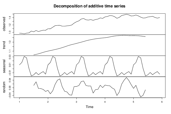
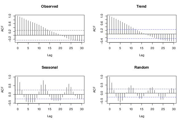
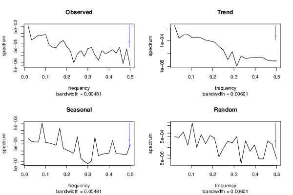
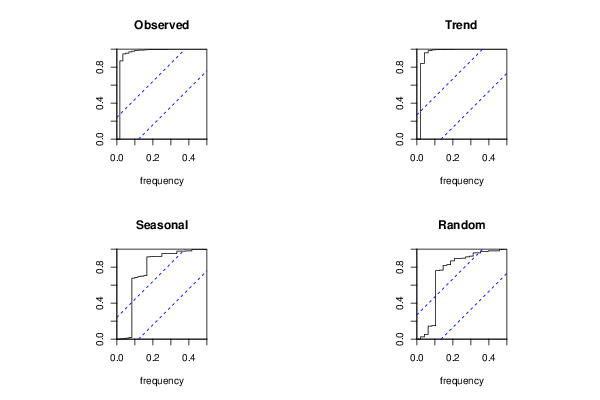
Title produced by software

Classical Decomposition

Date of computation

Thu, 22 May 2014 16:08:16 -0400

Cite this page as follows

Statistical Computations at FreeStatistics.org, Office for Research Development and Education, URL https://freestatistics.org/blog/index.php?v=date/2014/May/22/t1400789668mjwdj97cnm0l7nk.htm/, Retrieved Wed, 15 May 2024 06:06:41 +0000

Statistical Computations at FreeStatistics.org, Office for Research Development and Education, URL https://freestatistics.org/blog/index.php?pk=235141, Retrieved Wed, 15 May 2024 06:06:41 +0000

QR Codes:

Paste this QR Code to cite your computation.

Original text written by user:

IsPrivate?

No (this computation is public)

User-defined keywords

Estimated Impact

Family? (F = Feedback message, R = changed R code, M = changed R Module, P = changed Parameters, D = changed Data)

-       [Classical Decomposition] [] [2014-05-22 20:08:16] [d41d8cd98f00b204e9800998ecf8427e] [Current]

Feedback Forum

Post a new message

Dataseries X:

Download CSV

Histogram

Boxplots

Summary of computational transaction
Raw Input	view raw input (R code)
Raw Output	view raw output of R engine
Computing time	3 seconds
R Server	'Herman Ole Andreas Wold' @ wold.wessa.net

\begin{tabular}{lllllllll}
\hline
Summary of computational transaction \tabularnewline
Raw Input & view raw input (R code)  \tabularnewline
Raw Output & view raw output of R engine  \tabularnewline
Computing time & 3 seconds \tabularnewline
R Server & 'Herman Ole Andreas Wold' @ wold.wessa.net \tabularnewline
\hline
\end{tabular}
%Source: https://freestatistics.org/blog/index.php?pk=235141&T=0

[TABLE]
[ROW][C]Summary of computational transaction[/C][/ROW]
[ROW][C]Raw Input[/C][C]view raw input (R code) [/C][/ROW]
[ROW][C]Raw Output[/C][C]view raw output of R engine [/C][/ROW]
[ROW][C]Computing time[/C][C]3 seconds[/C][/ROW]
[ROW][C]R Server[/C][C]'Herman Ole Andreas Wold' @ wold.wessa.net[/C][/ROW]
[/TABLE]
Source: https://freestatistics.org/blog/index.php?pk=235141&T=0

Globally Unique Identifier (entire table): ba.freestatistics.org/blog/index.php?pk=235141&T=0

As an alternative you can also use a QR Code:

The GUIDs for individual cells are displayed in the table below:

Summary of computational transaction
Raw Input	view raw input (R code)
Raw Output	view raw output of R engine
Computing time	3 seconds
R Server	'Herman Ole Andreas Wold' @ wold.wessa.net

Classical Decomposition by Moving Averages
t	Observations	Fit	Trend	Seasonal	Random
1	0.978	NA	NA	0.0101016	NA
2	0.973	NA	NA	0.015987	NA
3	0.96	NA	NA	0.0312474	NA
4	0.978	NA	NA	0.0278828	NA
5	0.985	NA	NA	0.00116406	NA
6	1.035	NA	NA	-0.017638	NA
7	1.015	1.00275	1.01767	-0.0149193	0.0122526
8	1.05	1.01879	1.02783	-0.00904427	0.0312109
9	1.022	1.02587	1.04046	-0.0145859	-0.0038724
10	1.042	1.04618	1.05642	-0.0102318	-0.0041849
11	1.058	1.06666	1.07342	-0.0067526	-0.00866406
12	1.056	1.07521	1.08842	-0.0132109	-0.0192057
13	1.098	1.11139	1.10129	0.0101016	-0.0133932
14	1.097	1.12857	1.11258	0.015987	-0.0315703
15	1.139	1.15521	1.12396	0.0312474	-0.0162057
16	1.182	1.16422	1.13633	0.0278828	0.0177839
17	1.189	1.14933	1.14817	0.00116406	0.0396693
18	1.191	1.14457	1.16221	-0.017638	0.0464297
19	1.168	1.16333	1.17825	-0.0149193	0.00466927
20	1.168	1.18612	1.19517	-0.00904427	-0.0181224
21	1.177	1.19891	1.2135	-0.0145859	-0.0219141
22	1.184	1.22073	1.23096	-0.0102318	-0.0367266
23	1.2	1.23871	1.24546	-0.0067526	-0.0387057
24	1.251	1.24458	1.25779	-0.0132109	0.00641927
25	1.288	1.28135	1.27125	0.0101016	0.00664844
26	1.313	1.30136	1.28538	0.015987	0.011638
27	1.363	1.33041	1.29917	0.0312474	0.0325859
28	1.377	1.34159	1.31371	0.0278828	0.0354089
29	1.342	1.33029	1.32912	0.00116406	0.0117109
30	1.334	1.3249	1.34254	-0.017638	0.00909635
31	1.348	1.33854	1.35346	-0.0149193	0.00946094
32	1.327	1.35491	1.36396	-0.00904427	-0.0279141
33	1.349	1.35825	1.37283	-0.0145859	-0.0092474
34	1.361	1.36968	1.37992	-0.0102318	-0.0086849
35	1.393	1.37991	1.38667	-0.0067526	0.0130859
36	1.38	1.37908	1.39229	-0.0132109	0.000919271
37	1.421	1.40693	1.39683	0.0101016	0.0140651
38	1.432	1.42078	1.40479	0.015987	0.0112214
39	1.457	1.44671	1.41546	0.0312474	0.0102943
40	1.453	1.45397	1.42608	0.0278828	-0.000966146
41	1.428	1.43612	1.43496	0.00116406	-0.0081224
42	1.383	1.42353	1.44117	-0.017638	-0.0405286
43	1.408	1.43025	1.44517	-0.0149193	-0.0222474
44	1.458	1.43904	1.44808	-0.00904427	0.0189609
45	1.474	1.43483	1.44942	-0.0145859	0.0391693
46	1.491	1.43727	1.4475	-0.0102318	0.0537318
47	1.476	1.43758	1.44433	-0.0067526	0.0384193
48	1.446	1.43	1.44321	-0.0132109	0.0160026
49	1.451	1.45418	1.44408	0.0101016	-0.0031849
50	1.472	1.45915	1.44317	0.015987	0.0128464
51	1.449	1.47154	1.44029	0.0312474	-0.0225391
52	1.415	1.46309	1.43521	0.0278828	-0.0480911
53	1.39	1.42912	1.42796	0.00116406	-0.0391224
54	1.394	1.40486	1.4225	-0.017638	-0.010862
55	1.418	NA	NA	-0.0149193	NA
56	1.426	NA	NA	-0.00904427	NA
57	1.437	NA	NA	-0.0145859	NA
58	1.406	NA	NA	-0.0102318	NA
59	1.387	NA	NA	-0.0067526	NA
60	1.404	NA	NA	-0.0132109	NA

\begin{tabular}{lllllllll}
\hline
Classical Decomposition by Moving Averages \tabularnewline
t & Observations & Fit & Trend & Seasonal & Random \tabularnewline
1 & 0.978 & NA & NA & 0.0101016 & NA \tabularnewline
2 & 0.973 & NA & NA & 0.015987 & NA \tabularnewline
3 & 0.96 & NA & NA & 0.0312474 & NA \tabularnewline
4 & 0.978 & NA & NA & 0.0278828 & NA \tabularnewline
5 & 0.985 & NA & NA & 0.00116406 & NA \tabularnewline
6 & 1.035 & NA & NA & -0.017638 & NA \tabularnewline
7 & 1.015 & 1.00275 & 1.01767 & -0.0149193 & 0.0122526 \tabularnewline
8 & 1.05 & 1.01879 & 1.02783 & -0.00904427 & 0.0312109 \tabularnewline
9 & 1.022 & 1.02587 & 1.04046 & -0.0145859 & -0.0038724 \tabularnewline
10 & 1.042 & 1.04618 & 1.05642 & -0.0102318 & -0.0041849 \tabularnewline
11 & 1.058 & 1.06666 & 1.07342 & -0.0067526 & -0.00866406 \tabularnewline
12 & 1.056 & 1.07521 & 1.08842 & -0.0132109 & -0.0192057 \tabularnewline
13 & 1.098 & 1.11139 & 1.10129 & 0.0101016 & -0.0133932 \tabularnewline
14 & 1.097 & 1.12857 & 1.11258 & 0.015987 & -0.0315703 \tabularnewline
15 & 1.139 & 1.15521 & 1.12396 & 0.0312474 & -0.0162057 \tabularnewline
16 & 1.182 & 1.16422 & 1.13633 & 0.0278828 & 0.0177839 \tabularnewline
17 & 1.189 & 1.14933 & 1.14817 & 0.00116406 & 0.0396693 \tabularnewline
18 & 1.191 & 1.14457 & 1.16221 & -0.017638 & 0.0464297 \tabularnewline
19 & 1.168 & 1.16333 & 1.17825 & -0.0149193 & 0.00466927 \tabularnewline
20 & 1.168 & 1.18612 & 1.19517 & -0.00904427 & -0.0181224 \tabularnewline
21 & 1.177 & 1.19891 & 1.2135 & -0.0145859 & -0.0219141 \tabularnewline
22 & 1.184 & 1.22073 & 1.23096 & -0.0102318 & -0.0367266 \tabularnewline
23 & 1.2 & 1.23871 & 1.24546 & -0.0067526 & -0.0387057 \tabularnewline
24 & 1.251 & 1.24458 & 1.25779 & -0.0132109 & 0.00641927 \tabularnewline
25 & 1.288 & 1.28135 & 1.27125 & 0.0101016 & 0.00664844 \tabularnewline
26 & 1.313 & 1.30136 & 1.28538 & 0.015987 & 0.011638 \tabularnewline
27 & 1.363 & 1.33041 & 1.29917 & 0.0312474 & 0.0325859 \tabularnewline
28 & 1.377 & 1.34159 & 1.31371 & 0.0278828 & 0.0354089 \tabularnewline
29 & 1.342 & 1.33029 & 1.32912 & 0.00116406 & 0.0117109 \tabularnewline
30 & 1.334 & 1.3249 & 1.34254 & -0.017638 & 0.00909635 \tabularnewline
31 & 1.348 & 1.33854 & 1.35346 & -0.0149193 & 0.00946094 \tabularnewline
32 & 1.327 & 1.35491 & 1.36396 & -0.00904427 & -0.0279141 \tabularnewline
33 & 1.349 & 1.35825 & 1.37283 & -0.0145859 & -0.0092474 \tabularnewline
34 & 1.361 & 1.36968 & 1.37992 & -0.0102318 & -0.0086849 \tabularnewline
35 & 1.393 & 1.37991 & 1.38667 & -0.0067526 & 0.0130859 \tabularnewline
36 & 1.38 & 1.37908 & 1.39229 & -0.0132109 & 0.000919271 \tabularnewline
37 & 1.421 & 1.40693 & 1.39683 & 0.0101016 & 0.0140651 \tabularnewline
38 & 1.432 & 1.42078 & 1.40479 & 0.015987 & 0.0112214 \tabularnewline
39 & 1.457 & 1.44671 & 1.41546 & 0.0312474 & 0.0102943 \tabularnewline
40 & 1.453 & 1.45397 & 1.42608 & 0.0278828 & -0.000966146 \tabularnewline
41 & 1.428 & 1.43612 & 1.43496 & 0.00116406 & -0.0081224 \tabularnewline
42 & 1.383 & 1.42353 & 1.44117 & -0.017638 & -0.0405286 \tabularnewline
43 & 1.408 & 1.43025 & 1.44517 & -0.0149193 & -0.0222474 \tabularnewline
44 & 1.458 & 1.43904 & 1.44808 & -0.00904427 & 0.0189609 \tabularnewline
45 & 1.474 & 1.43483 & 1.44942 & -0.0145859 & 0.0391693 \tabularnewline
46 & 1.491 & 1.43727 & 1.4475 & -0.0102318 & 0.0537318 \tabularnewline
47 & 1.476 & 1.43758 & 1.44433 & -0.0067526 & 0.0384193 \tabularnewline
48 & 1.446 & 1.43 & 1.44321 & -0.0132109 & 0.0160026 \tabularnewline
49 & 1.451 & 1.45418 & 1.44408 & 0.0101016 & -0.0031849 \tabularnewline
50 & 1.472 & 1.45915 & 1.44317 & 0.015987 & 0.0128464 \tabularnewline
51 & 1.449 & 1.47154 & 1.44029 & 0.0312474 & -0.0225391 \tabularnewline
52 & 1.415 & 1.46309 & 1.43521 & 0.0278828 & -0.0480911 \tabularnewline
53 & 1.39 & 1.42912 & 1.42796 & 0.00116406 & -0.0391224 \tabularnewline
54 & 1.394 & 1.40486 & 1.4225 & -0.017638 & -0.010862 \tabularnewline
55 & 1.418 & NA & NA & -0.0149193 & NA \tabularnewline
56 & 1.426 & NA & NA & -0.00904427 & NA \tabularnewline
57 & 1.437 & NA & NA & -0.0145859 & NA \tabularnewline
58 & 1.406 & NA & NA & -0.0102318 & NA \tabularnewline
59 & 1.387 & NA & NA & -0.0067526 & NA \tabularnewline
60 & 1.404 & NA & NA & -0.0132109 & NA \tabularnewline
\hline
\end{tabular}
%Source: https://freestatistics.org/blog/index.php?pk=235141&T=1

[TABLE]
[ROW][C]Classical Decomposition by Moving Averages[/C][/ROW]
[ROW][C]t[/C][C]Observations[/C][C]Fit[/C][C]Trend[/C][C]Seasonal[/C][C]Random[/C][/ROW]
[ROW][C]1[/C][C]0.978[/C][C]NA[/C][C]NA[/C][C]0.0101016[/C][C]NA[/C][/ROW]
[ROW][C]2[/C][C]0.973[/C][C]NA[/C][C]NA[/C][C]0.015987[/C][C]NA[/C][/ROW]
[ROW][C]3[/C][C]0.96[/C][C]NA[/C][C]NA[/C][C]0.0312474[/C][C]NA[/C][/ROW]
[ROW][C]4[/C][C]0.978[/C][C]NA[/C][C]NA[/C][C]0.0278828[/C][C]NA[/C][/ROW]
[ROW][C]5[/C][C]0.985[/C][C]NA[/C][C]NA[/C][C]0.00116406[/C][C]NA[/C][/ROW]
[ROW][C]6[/C][C]1.035[/C][C]NA[/C][C]NA[/C][C]-0.017638[/C][C]NA[/C][/ROW]
[ROW][C]7[/C][C]1.015[/C][C]1.00275[/C][C]1.01767[/C][C]-0.0149193[/C][C]0.0122526[/C][/ROW]
[ROW][C]8[/C][C]1.05[/C][C]1.01879[/C][C]1.02783[/C][C]-0.00904427[/C][C]0.0312109[/C][/ROW]
[ROW][C]9[/C][C]1.022[/C][C]1.02587[/C][C]1.04046[/C][C]-0.0145859[/C][C]-0.0038724[/C][/ROW]
[ROW][C]10[/C][C]1.042[/C][C]1.04618[/C][C]1.05642[/C][C]-0.0102318[/C][C]-0.0041849[/C][/ROW]
[ROW][C]11[/C][C]1.058[/C][C]1.06666[/C][C]1.07342[/C][C]-0.0067526[/C][C]-0.00866406[/C][/ROW]
[ROW][C]12[/C][C]1.056[/C][C]1.07521[/C][C]1.08842[/C][C]-0.0132109[/C][C]-0.0192057[/C][/ROW]
[ROW][C]13[/C][C]1.098[/C][C]1.11139[/C][C]1.10129[/C][C]0.0101016[/C][C]-0.0133932[/C][/ROW]
[ROW][C]14[/C][C]1.097[/C][C]1.12857[/C][C]1.11258[/C][C]0.015987[/C][C]-0.0315703[/C][/ROW]
[ROW][C]15[/C][C]1.139[/C][C]1.15521[/C][C]1.12396[/C][C]0.0312474[/C][C]-0.0162057[/C][/ROW]
[ROW][C]16[/C][C]1.182[/C][C]1.16422[/C][C]1.13633[/C][C]0.0278828[/C][C]0.0177839[/C][/ROW]
[ROW][C]17[/C][C]1.189[/C][C]1.14933[/C][C]1.14817[/C][C]0.00116406[/C][C]0.0396693[/C][/ROW]
[ROW][C]18[/C][C]1.191[/C][C]1.14457[/C][C]1.16221[/C][C]-0.017638[/C][C]0.0464297[/C][/ROW]
[ROW][C]19[/C][C]1.168[/C][C]1.16333[/C][C]1.17825[/C][C]-0.0149193[/C][C]0.00466927[/C][/ROW]
[ROW][C]20[/C][C]1.168[/C][C]1.18612[/C][C]1.19517[/C][C]-0.00904427[/C][C]-0.0181224[/C][/ROW]
[ROW][C]21[/C][C]1.177[/C][C]1.19891[/C][C]1.2135[/C][C]-0.0145859[/C][C]-0.0219141[/C][/ROW]
[ROW][C]22[/C][C]1.184[/C][C]1.22073[/C][C]1.23096[/C][C]-0.0102318[/C][C]-0.0367266[/C][/ROW]
[ROW][C]23[/C][C]1.2[/C][C]1.23871[/C][C]1.24546[/C][C]-0.0067526[/C][C]-0.0387057[/C][/ROW]
[ROW][C]24[/C][C]1.251[/C][C]1.24458[/C][C]1.25779[/C][C]-0.0132109[/C][C]0.00641927[/C][/ROW]
[ROW][C]25[/C][C]1.288[/C][C]1.28135[/C][C]1.27125[/C][C]0.0101016[/C][C]0.00664844[/C][/ROW]
[ROW][C]26[/C][C]1.313[/C][C]1.30136[/C][C]1.28538[/C][C]0.015987[/C][C]0.011638[/C][/ROW]
[ROW][C]27[/C][C]1.363[/C][C]1.33041[/C][C]1.29917[/C][C]0.0312474[/C][C]0.0325859[/C][/ROW]
[ROW][C]28[/C][C]1.377[/C][C]1.34159[/C][C]1.31371[/C][C]0.0278828[/C][C]0.0354089[/C][/ROW]
[ROW][C]29[/C][C]1.342[/C][C]1.33029[/C][C]1.32912[/C][C]0.00116406[/C][C]0.0117109[/C][/ROW]
[ROW][C]30[/C][C]1.334[/C][C]1.3249[/C][C]1.34254[/C][C]-0.017638[/C][C]0.00909635[/C][/ROW]
[ROW][C]31[/C][C]1.348[/C][C]1.33854[/C][C]1.35346[/C][C]-0.0149193[/C][C]0.00946094[/C][/ROW]
[ROW][C]32[/C][C]1.327[/C][C]1.35491[/C][C]1.36396[/C][C]-0.00904427[/C][C]-0.0279141[/C][/ROW]
[ROW][C]33[/C][C]1.349[/C][C]1.35825[/C][C]1.37283[/C][C]-0.0145859[/C][C]-0.0092474[/C][/ROW]
[ROW][C]34[/C][C]1.361[/C][C]1.36968[/C][C]1.37992[/C][C]-0.0102318[/C][C]-0.0086849[/C][/ROW]
[ROW][C]35[/C][C]1.393[/C][C]1.37991[/C][C]1.38667[/C][C]-0.0067526[/C][C]0.0130859[/C][/ROW]
[ROW][C]36[/C][C]1.38[/C][C]1.37908[/C][C]1.39229[/C][C]-0.0132109[/C][C]0.000919271[/C][/ROW]
[ROW][C]37[/C][C]1.421[/C][C]1.40693[/C][C]1.39683[/C][C]0.0101016[/C][C]0.0140651[/C][/ROW]
[ROW][C]38[/C][C]1.432[/C][C]1.42078[/C][C]1.40479[/C][C]0.015987[/C][C]0.0112214[/C][/ROW]
[ROW][C]39[/C][C]1.457[/C][C]1.44671[/C][C]1.41546[/C][C]0.0312474[/C][C]0.0102943[/C][/ROW]
[ROW][C]40[/C][C]1.453[/C][C]1.45397[/C][C]1.42608[/C][C]0.0278828[/C][C]-0.000966146[/C][/ROW]
[ROW][C]41[/C][C]1.428[/C][C]1.43612[/C][C]1.43496[/C][C]0.00116406[/C][C]-0.0081224[/C][/ROW]
[ROW][C]42[/C][C]1.383[/C][C]1.42353[/C][C]1.44117[/C][C]-0.017638[/C][C]-0.0405286[/C][/ROW]
[ROW][C]43[/C][C]1.408[/C][C]1.43025[/C][C]1.44517[/C][C]-0.0149193[/C][C]-0.0222474[/C][/ROW]
[ROW][C]44[/C][C]1.458[/C][C]1.43904[/C][C]1.44808[/C][C]-0.00904427[/C][C]0.0189609[/C][/ROW]
[ROW][C]45[/C][C]1.474[/C][C]1.43483[/C][C]1.44942[/C][C]-0.0145859[/C][C]0.0391693[/C][/ROW]
[ROW][C]46[/C][C]1.491[/C][C]1.43727[/C][C]1.4475[/C][C]-0.0102318[/C][C]0.0537318[/C][/ROW]
[ROW][C]47[/C][C]1.476[/C][C]1.43758[/C][C]1.44433[/C][C]-0.0067526[/C][C]0.0384193[/C][/ROW]
[ROW][C]48[/C][C]1.446[/C][C]1.43[/C][C]1.44321[/C][C]-0.0132109[/C][C]0.0160026[/C][/ROW]
[ROW][C]49[/C][C]1.451[/C][C]1.45418[/C][C]1.44408[/C][C]0.0101016[/C][C]-0.0031849[/C][/ROW]
[ROW][C]50[/C][C]1.472[/C][C]1.45915[/C][C]1.44317[/C][C]0.015987[/C][C]0.0128464[/C][/ROW]
[ROW][C]51[/C][C]1.449[/C][C]1.47154[/C][C]1.44029[/C][C]0.0312474[/C][C]-0.0225391[/C][/ROW]
[ROW][C]52[/C][C]1.415[/C][C]1.46309[/C][C]1.43521[/C][C]0.0278828[/C][C]-0.0480911[/C][/ROW]
[ROW][C]53[/C][C]1.39[/C][C]1.42912[/C][C]1.42796[/C][C]0.00116406[/C][C]-0.0391224[/C][/ROW]
[ROW][C]54[/C][C]1.394[/C][C]1.40486[/C][C]1.4225[/C][C]-0.017638[/C][C]-0.010862[/C][/ROW]
[ROW][C]55[/C][C]1.418[/C][C]NA[/C][C]NA[/C][C]-0.0149193[/C][C]NA[/C][/ROW]
[ROW][C]56[/C][C]1.426[/C][C]NA[/C][C]NA[/C][C]-0.00904427[/C][C]NA[/C][/ROW]
[ROW][C]57[/C][C]1.437[/C][C]NA[/C][C]NA[/C][C]-0.0145859[/C][C]NA[/C][/ROW]
[ROW][C]58[/C][C]1.406[/C][C]NA[/C][C]NA[/C][C]-0.0102318[/C][C]NA[/C][/ROW]
[ROW][C]59[/C][C]1.387[/C][C]NA[/C][C]NA[/C][C]-0.0067526[/C][C]NA[/C][/ROW]
[ROW][C]60[/C][C]1.404[/C][C]NA[/C][C]NA[/C][C]-0.0132109[/C][C]NA[/C][/ROW]
[/TABLE]
Source: https://freestatistics.org/blog/index.php?pk=235141&T=1

Globally Unique Identifier (entire table): ba.freestatistics.org/blog/index.php?pk=235141&T=1

As an alternative you can also use a QR Code:

The GUIDs for individual cells are displayed in the table below:

Classical Decomposition by Moving Averages
t	Observations	Fit	Trend	Seasonal	Random
1	0.978	NA	NA	0.0101016	NA
2	0.973	NA	NA	0.015987	NA
3	0.96	NA	NA	0.0312474	NA
4	0.978	NA	NA	0.0278828	NA
5	0.985	NA	NA	0.00116406	NA
6	1.035	NA	NA	-0.017638	NA
7	1.015	1.00275	1.01767	-0.0149193	0.0122526
8	1.05	1.01879	1.02783	-0.00904427	0.0312109
9	1.022	1.02587	1.04046	-0.0145859	-0.0038724
10	1.042	1.04618	1.05642	-0.0102318	-0.0041849
11	1.058	1.06666	1.07342	-0.0067526	-0.00866406
12	1.056	1.07521	1.08842	-0.0132109	-0.0192057
13	1.098	1.11139	1.10129	0.0101016	-0.0133932
14	1.097	1.12857	1.11258	0.015987	-0.0315703
15	1.139	1.15521	1.12396	0.0312474	-0.0162057
16	1.182	1.16422	1.13633	0.0278828	0.0177839
17	1.189	1.14933	1.14817	0.00116406	0.0396693
18	1.191	1.14457	1.16221	-0.017638	0.0464297
19	1.168	1.16333	1.17825	-0.0149193	0.00466927
20	1.168	1.18612	1.19517	-0.00904427	-0.0181224
21	1.177	1.19891	1.2135	-0.0145859	-0.0219141
22	1.184	1.22073	1.23096	-0.0102318	-0.0367266
23	1.2	1.23871	1.24546	-0.0067526	-0.0387057
24	1.251	1.24458	1.25779	-0.0132109	0.00641927
25	1.288	1.28135	1.27125	0.0101016	0.00664844
26	1.313	1.30136	1.28538	0.015987	0.011638
27	1.363	1.33041	1.29917	0.0312474	0.0325859
28	1.377	1.34159	1.31371	0.0278828	0.0354089
29	1.342	1.33029	1.32912	0.00116406	0.0117109
30	1.334	1.3249	1.34254	-0.017638	0.00909635
31	1.348	1.33854	1.35346	-0.0149193	0.00946094
32	1.327	1.35491	1.36396	-0.00904427	-0.0279141
33	1.349	1.35825	1.37283	-0.0145859	-0.0092474
34	1.361	1.36968	1.37992	-0.0102318	-0.0086849
35	1.393	1.37991	1.38667	-0.0067526	0.0130859
36	1.38	1.37908	1.39229	-0.0132109	0.000919271
37	1.421	1.40693	1.39683	0.0101016	0.0140651
38	1.432	1.42078	1.40479	0.015987	0.0112214
39	1.457	1.44671	1.41546	0.0312474	0.0102943
40	1.453	1.45397	1.42608	0.0278828	-0.000966146
41	1.428	1.43612	1.43496	0.00116406	-0.0081224
42	1.383	1.42353	1.44117	-0.017638	-0.0405286
43	1.408	1.43025	1.44517	-0.0149193	-0.0222474
44	1.458	1.43904	1.44808	-0.00904427	0.0189609
45	1.474	1.43483	1.44942	-0.0145859	0.0391693
46	1.491	1.43727	1.4475	-0.0102318	0.0537318
47	1.476	1.43758	1.44433	-0.0067526	0.0384193
48	1.446	1.43	1.44321	-0.0132109	0.0160026
49	1.451	1.45418	1.44408	0.0101016	-0.0031849
50	1.472	1.45915	1.44317	0.015987	0.0128464
51	1.449	1.47154	1.44029	0.0312474	-0.0225391
52	1.415	1.46309	1.43521	0.0278828	-0.0480911
53	1.39	1.42912	1.42796	0.00116406	-0.0391224
54	1.394	1.40486	1.4225	-0.017638	-0.010862
55	1.418	NA	NA	-0.0149193	NA
56	1.426	NA	NA	-0.00904427	NA
57	1.437	NA	NA	-0.0145859	NA
58	1.406	NA	NA	-0.0102318	NA
59	1.387	NA	NA	-0.0067526	NA
60	1.404	NA	NA	-0.0132109	NA

Figure 1

PNG link

Postscript link

PDF link

Figure 2

PNG link

Postscript link

PDF link

Figure 3

PNG link

Postscript link

PDF link

Figure 4

PNG link

Postscript link

PDF link

Parameters (Session):

par1 = additive ; par2 = 12 ;

Parameters (R input):

par1 = additive ; par2 = 12 ;

R code (references can be found in the software module):

par2 <- as.numeric(par2)
x <- ts(x,freq=par2)
m <- decompose(x,type=par1)
m$figure
bitmap(file='test1.png')
plot(m)
dev.off()
mylagmax <- length(x)/2
bitmap(file='test2.png')
op <- par(mfrow = c(2,2))
acf(as.numeric(x),lag.max = mylagmax,main='Observed')
acf(as.numeric(m$trend),na.action=na.pass,lag.max = mylagmax,main='Trend')
acf(as.numeric(m$seasonal),na.action=na.pass,lag.max = mylagmax,main='Seasonal')
acf(as.numeric(m$random),na.action=na.pass,lag.max = mylagmax,main='Random')
par(op)
dev.off()
bitmap(file='test3.png')
op <- par(mfrow = c(2,2))
spectrum(as.numeric(x),main='Observed')
spectrum(as.numeric(m$trend[!is.na(m$trend)]),main='Trend')
spectrum(as.numeric(m$seasonal[!is.na(m$seasonal)]),main='Seasonal')
spectrum(as.numeric(m$random[!is.na(m$random)]),main='Random')
par(op)
dev.off()
bitmap(file='test4.png')
op <- par(mfrow = c(2,2))
cpgram(as.numeric(x),main='Observed')
cpgram(as.numeric(m$trend[!is.na(m$trend)]),main='Trend')
cpgram(as.numeric(m$seasonal[!is.na(m$seasonal)]),main='Seasonal')
cpgram(as.numeric(m$random[!is.na(m$random)]),main='Random')
par(op)
dev.off()
load(file='createtable')
a<-table.start()
a<-table.row.start(a)
a<-table.element(a,'Classical Decomposition by Moving Averages',6,TRUE)
a<-table.row.end(a)
a<-table.row.start(a)
a<-table.element(a,'t',header=TRUE)
a<-table.element(a,'Observations',header=TRUE)
a<-table.element(a,'Fit',header=TRUE)
a<-table.element(a,'Trend',header=TRUE)
a<-table.element(a,'Seasonal',header=TRUE)
a<-table.element(a,'Random',header=TRUE)
a<-table.row.end(a)
for (i in 1:length(m$trend)) {
a<-table.row.start(a)
a<-table.element(a,i,header=TRUE)
a<-table.element(a,x[i])
if (par1 == 'additive') a<-table.element(a,signif(m$trend[i]+m$seasonal[i],6)) else a<-table.element(a,signif(m$trend[i]*m$seasonal[i],6))
a<-table.element(a,signif(m$trend[i],6))
a<-table.element(a,signif(m$seasonal[i],6))
a<-table.element(a,signif(m$random[i],6))
a<-table.row.end(a)
}
a<-table.end(a)
table.save(a,file='mytable.tab')

Free Statistics

Description of Statistical Computation

Tree of Dependent Computations

Dataset

Tables (Output of Computation)

Figures (Output of Computation)

Input Parameters & R Code