Free Statistics
of Irreproducible Research!
Description of Statistical Computation | |||||||||||||||||||||||||||||||||||||||||||||||||||||||||||||||||||||||||||||||||
|---|---|---|---|---|---|---|---|---|---|---|---|---|---|---|---|---|---|---|---|---|---|---|---|---|---|---|---|---|---|---|---|---|---|---|---|---|---|---|---|---|---|---|---|---|---|---|---|---|---|---|---|---|---|---|---|---|---|---|---|---|---|---|---|---|---|---|---|---|---|---|---|---|---|---|---|---|---|---|---|---|---|
| Author's title | |||||||||||||||||||||||||||||||||||||||||||||||||||||||||||||||||||||||||||||||||
| Author | *Unverified author* | ||||||||||||||||||||||||||||||||||||||||||||||||||||||||||||||||||||||||||||||||
| R Software Module | rwasp_bootstrapplot.wasp | ||||||||||||||||||||||||||||||||||||||||||||||||||||||||||||||||||||||||||||||||
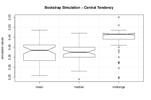
| Title produced by software | Blocked Bootstrap Plot - Central Tendency | ||||||||||||||||||||||||||||||||||||||||||||||||||||||||||||||||||||||||||||||||
| Date of computation | Mon, 17 Nov 2014 10:07:50 +0000 | ||||||||||||||||||||||||||||||||||||||||||||||||||||||||||||||||||||||||||||||||
| Cite this page as follows | Statistical Computations at FreeStatistics.org, Office for Research Development and Education, URL https://freestatistics.org/blog/index.php?v=date/2014/Nov/17/t14162188825vo5dtin0smsii5.htm/, Retrieved Wed, 15 May 2024 20:16:39 +0000 | ||||||||||||||||||||||||||||||||||||||||||||||||||||||||||||||||||||||||||||||||
| Statistical Computations at FreeStatistics.org, Office for Research Development and Education, URL https://freestatistics.org/blog/index.php?pk=255383, Retrieved Wed, 15 May 2024 20:16:39 +0000 | |||||||||||||||||||||||||||||||||||||||||||||||||||||||||||||||||||||||||||||||||
| QR Codes: | |||||||||||||||||||||||||||||||||||||||||||||||||||||||||||||||||||||||||||||||||
|
| |||||||||||||||||||||||||||||||||||||||||||||||||||||||||||||||||||||||||||||||||
| Original text written by user: | |||||||||||||||||||||||||||||||||||||||||||||||||||||||||||||||||||||||||||||||||
| IsPrivate? | No (this computation is public) | ||||||||||||||||||||||||||||||||||||||||||||||||||||||||||||||||||||||||||||||||
| User-defined keywords | |||||||||||||||||||||||||||||||||||||||||||||||||||||||||||||||||||||||||||||||||
| Estimated Impact | 118 | ||||||||||||||||||||||||||||||||||||||||||||||||||||||||||||||||||||||||||||||||
Tree of Dependent Computations | |||||||||||||||||||||||||||||||||||||||||||||||||||||||||||||||||||||||||||||||||
| Family? (F = Feedback message, R = changed R code, M = changed R Module, P = changed Parameters, D = changed Data) | |||||||||||||||||||||||||||||||||||||||||||||||||||||||||||||||||||||||||||||||||
| - [Blocked Bootstrap Plot - Central Tendency] [] [2014-11-17 10:07:50] [f2e79deb6e51141b138dd10990a8e48d] [Current] | |||||||||||||||||||||||||||||||||||||||||||||||||||||||||||||||||||||||||||||||||
| Feedback Forum | |||||||||||||||||||||||||||||||||||||||||||||||||||||||||||||||||||||||||||||||||
Post a new message | |||||||||||||||||||||||||||||||||||||||||||||||||||||||||||||||||||||||||||||||||
Dataset | |||||||||||||||||||||||||||||||||||||||||||||||||||||||||||||||||||||||||||||||||
| Dataseries X: | |||||||||||||||||||||||||||||||||||||||||||||||||||||||||||||||||||||||||||||||||
5,06 5,05 5,05 5,04 5,06 5,07 5,09 5,08 5,09 5,09 5,09 5,1 5,12 5,14 5,14 5,14 5,13 5,15 5,16 5,17 5,17 5,18 5,21 5,19 5,22 5,24 5,21 5,24 5,28 5,3 5,32 5,32 5,29 5,3 5,32 5,31 5,35 5,36 5,33 5,35 5,35 5,35 5,37 5,39 5,4 5,39 5,4 5,4 5,4 5,38 5,32 5,36 5,35 5,39 5,4 5,41 5,36 5,38 5,41 5,35 5,4 5,41 5,42 5,41 5,41 5,42 5,4 5,42 5,41 5,34 5,46 5,45 5,47 5,48 5,43 5,5 5,51 5,51 5,52 5,55 5,55 5,48 5,61 5,59 5,68 5,71 5,68 5,7 5,76 5,78 5,77 5,85 5,82 5,84 5,89 5,84 | |||||||||||||||||||||||||||||||||||||||||||||||||||||||||||||||||||||||||||||||||
Tables (Output of Computation) | |||||||||||||||||||||||||||||||||||||||||||||||||||||||||||||||||||||||||||||||||
| |||||||||||||||||||||||||||||||||||||||||||||||||||||||||||||||||||||||||||||||||
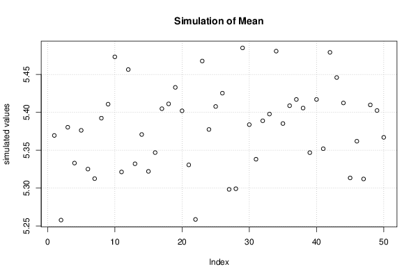
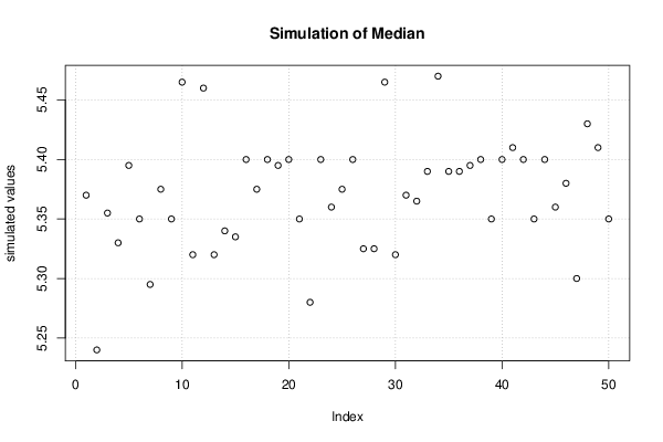
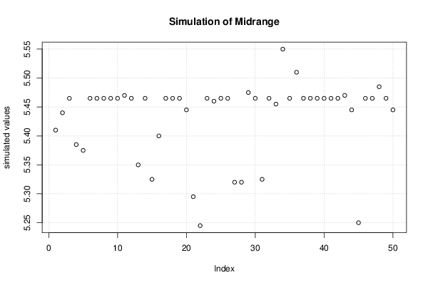
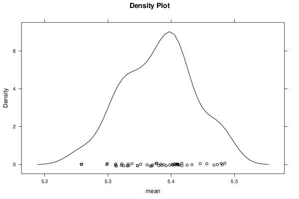
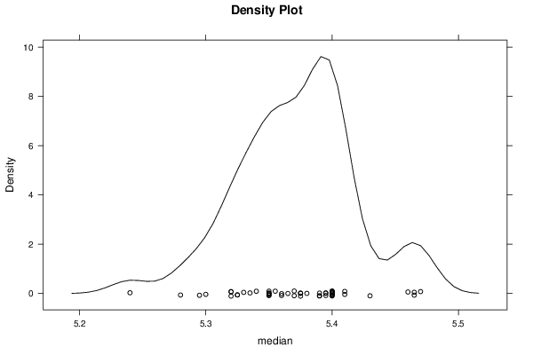
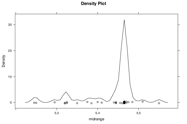
Figures (Output of Computation) | |||||||||||||||||||||||||||||||||||||||||||||||||||||||||||||||||||||||||||||||||
Input Parameters & R Code | |||||||||||||||||||||||||||||||||||||||||||||||||||||||||||||||||||||||||||||||||
| Parameters (Session): | |||||||||||||||||||||||||||||||||||||||||||||||||||||||||||||||||||||||||||||||||
| par1 = 50 ; par2 = 12 ; | |||||||||||||||||||||||||||||||||||||||||||||||||||||||||||||||||||||||||||||||||
| Parameters (R input): | |||||||||||||||||||||||||||||||||||||||||||||||||||||||||||||||||||||||||||||||||
| par1 = 50 ; par2 = 12 ; | |||||||||||||||||||||||||||||||||||||||||||||||||||||||||||||||||||||||||||||||||
| R code (references can be found in the software module): | |||||||||||||||||||||||||||||||||||||||||||||||||||||||||||||||||||||||||||||||||
par1 <- as.numeric(par1) | |||||||||||||||||||||||||||||||||||||||||||||||||||||||||||||||||||||||||||||||||