Free Statistics

of Irreproducible Research!

Author's title

Author*Unverified author*
R Software Modulerwasp_density.wasp
Title produced by softwareKernel Density Estimation
Date of computationFri, 26 Sep 2014 15:37:29 +0100
Cite this page as followsStatistical Computations at FreeStatistics.org, Office for Research Development and Education, URL https://freestatistics.org/blog/index.php?v=date/2014/Sep/26/t1411742389xw36ispmcdxufiv.htm/, Retrieved Mon, 13 May 2024 00:16:43 +0000
Statistical Computations at FreeStatistics.org, Office for Research Development and Education, URL https://freestatistics.org/blog/index.php?pk=236347, Retrieved Mon, 13 May 2024 00:16:43 +0000
QR Codes:

Original text written by user:
IsPrivate?No (this computation is public)
User-defined keywords
Estimated Impact95
Family? (F = Feedback message, R = changed R code, M = changed R Module, P = changed Parameters, D = changed Data)
-     [Univariate Data Series] [] [2014-09-20 09:08:01] [52bcad4f2450da6a1432dda11dba2117]
- RMPD    [Kernel Density Estimation] [] [2014-09-26 14:37:29] [c53b0bb515ebe5f6f1384250cc1174dd] [Current]
Feedback Forum

Post a new message
Dataseries X:
246.78
247.91
247.99
248.6
248.68
248.75
248.75
249.03
249.05
249.57
249.35
249.46
249.46
250.82
254.19
255.18
256.68
256.73
256.73
257.39
257.78
258.67
258.71
258.91
258.91
261.38
262.42
262.77
263.24
262.83
262.83
263.09
263.6
265.68
266.08
266.28
266.28
269.14
270.96
272.97
273.13
274.73
274.73
274.59
275.15
275.16
275.38
275.4
275.4
275.71
275.21
279.04
279.1
279.11
279.11
279.02
279.3
279.34
279.36
279.39
279.39
280.21
283
284.33
285.15
284.21
284.21
284.17
286.28
286.95
287.12
287.34


Summary of computational transaction
Raw Inputview raw input (R code)
Raw Outputview raw output of R engine
Computing time3 seconds
R Server'Gertrude Mary Cox' @ cox.wessa.net

\begin{tabular}{lllllllll}
\hline
Summary of computational transaction \tabularnewline
Raw Input & view raw input (R code)  \tabularnewline
Raw Output & view raw output of R engine  \tabularnewline
Computing time & 3 seconds \tabularnewline
R Server & 'Gertrude Mary Cox' @ cox.wessa.net \tabularnewline
\hline
\end{tabular}
%Source: https://freestatistics.org/blog/index.php?pk=236347&T=0

[TABLE]
[ROW][C]Summary of computational transaction[/C][/ROW]
[ROW][C]Raw Input[/C][C]view raw input (R code) [/C][/ROW]
[ROW][C]Raw Output[/C][C]view raw output of R engine [/C][/ROW]
[ROW][C]Computing time[/C][C]3 seconds[/C][/ROW]
[ROW][C]R Server[/C][C]'Gertrude Mary Cox' @ cox.wessa.net[/C][/ROW]
[/TABLE]
Source: https://freestatistics.org/blog/index.php?pk=236347&T=0

Globally Unique Identifier (entire table): ba.freestatistics.org/blog/index.php?pk=236347&T=0

As an alternative you can also use a QR Code:  

The GUIDs for individual cells are displayed in the table below:

Summary of computational transaction
Raw Inputview raw input (R code)
Raw Outputview raw output of R engine
Computing time3 seconds
R Server'Gertrude Mary Cox' @ cox.wessa.net


Properties of Density Trace
Bandwidth4.893112926556
#Observations72

\begin{tabular}{lllllllll}
\hline
Properties of Density Trace \tabularnewline
Bandwidth & 4.893112926556 \tabularnewline
#Observations & 72 \tabularnewline
\hline
\end{tabular}
%Source: https://freestatistics.org/blog/index.php?pk=236347&T=1

[TABLE]
[ROW][C]Properties of Density Trace[/C][/ROW]
[ROW][C]Bandwidth[/C][C]4.893112926556[/C][/ROW]
[ROW][C]#Observations[/C][C]72[/C][/ROW]
[/TABLE]
Source: https://freestatistics.org/blog/index.php?pk=236347&T=1

Globally Unique Identifier (entire table): ba.freestatistics.org/blog/index.php?pk=236347&T=1

As an alternative you can also use a QR Code:  

The GUIDs for individual cells are displayed in the table below:

Properties of Density Trace
Bandwidth4.893112926556
#Observations72


Maximum Density Values
Kernelx-valuemax. density
Gaussian277.9377590332040.0277817543827249
Epanechnikov278.8955491367560.0269740770646623
Rectangular279.1692034520570.0278154416054717
Triangular279.1692034520570.0275926088628522
Biweight278.6218948214560.0270451430180316
Cosine278.4850676638050.027136542753213
Optcosine278.8955491367560.0269808963511329

\begin{tabular}{lllllllll}
\hline
Maximum Density Values \tabularnewline
Kernel & x-value & max. density \tabularnewline
Gaussian & 277.937759033204 & 0.0277817543827249 \tabularnewline
Epanechnikov & 278.895549136756 & 0.0269740770646623 \tabularnewline
Rectangular & 279.169203452057 & 0.0278154416054717 \tabularnewline
Triangular & 279.169203452057 & 0.0275926088628522 \tabularnewline
Biweight & 278.621894821456 & 0.0270451430180316 \tabularnewline
Cosine & 278.485067663805 & 0.027136542753213 \tabularnewline
Optcosine & 278.895549136756 & 0.0269808963511329 \tabularnewline
\hline
\end{tabular}
%Source: https://freestatistics.org/blog/index.php?pk=236347&T=2

[TABLE]
[ROW][C]Maximum Density Values[/C][/ROW]
[ROW][C]Kernel[/C][C]x-value[/C][C]max. density[/C][/ROW]
[ROW][C]Gaussian[/C][C]277.937759033204[/C][C]0.0277817543827249[/C][/ROW]
[ROW][C]Epanechnikov[/C][C]278.895549136756[/C][C]0.0269740770646623[/C][/ROW]
[ROW][C]Rectangular[/C][C]279.169203452057[/C][C]0.0278154416054717[/C][/ROW]
[ROW][C]Triangular[/C][C]279.169203452057[/C][C]0.0275926088628522[/C][/ROW]
[ROW][C]Biweight[/C][C]278.621894821456[/C][C]0.0270451430180316[/C][/ROW]
[ROW][C]Cosine[/C][C]278.485067663805[/C][C]0.027136542753213[/C][/ROW]
[ROW][C]Optcosine[/C][C]278.895549136756[/C][C]0.0269808963511329[/C][/ROW]
[/TABLE]
Source: https://freestatistics.org/blog/index.php?pk=236347&T=2

Globally Unique Identifier (entire table): ba.freestatistics.org/blog/index.php?pk=236347&T=2

As an alternative you can also use a QR Code:  

The GUIDs for individual cells are displayed in the table below:

Maximum Density Values
Kernelx-valuemax. density
Gaussian277.9377590332040.0277817543827249
Epanechnikov278.8955491367560.0269740770646623
Rectangular279.1692034520570.0278154416054717
Triangular279.1692034520570.0275926088628522
Biweight278.6218948214560.0270451430180316
Cosine278.4850676638050.027136542753213
Optcosine278.8955491367560.0269808963511329


Parameters (Session):
par1 = 0 ; par2 = no ; par3 = 512 ;
Parameters (R input):
par1 = 0 ; par2 = no ; par3 = 512 ;
R code (references can be found in the software module):
if (par1 == '0') bw <- 'nrd0'
if (par1 != '0') bw <- as.numeric(par1)
par3 <- as.numeric(par3)
mydensity <- array(NA, dim=c(par3,8))
bitmap(file='density1.png')
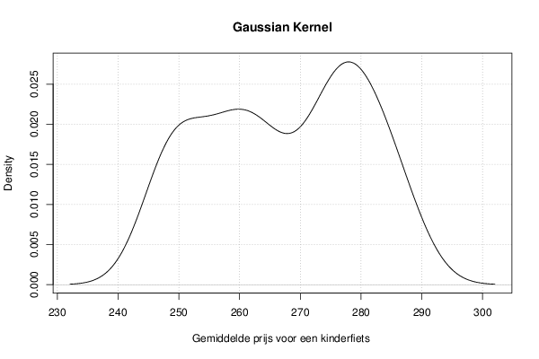
mydensity1<-density(x,bw=bw,kernel='gaussian',na.rm=TRUE)
mydensity[,8] = signif(mydensity1$x,3)
mydensity[,1] = signif(mydensity1$y,3)
plot(mydensity1,main='Gaussian Kernel',xlab=xlab,ylab=ylab)
grid()
dev.off()
mydensity1
bitmap(file='density2.png')
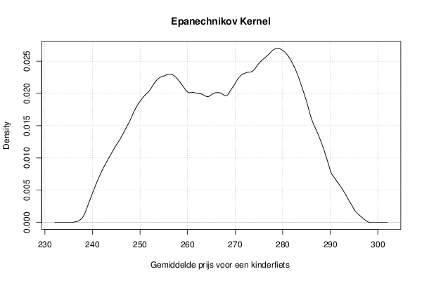
mydensity2<-density(x,bw=bw,kernel='epanechnikov',na.rm=TRUE)
mydensity[,2] = signif(mydensity2$y,3)
plot(mydensity2,main='Epanechnikov Kernel',xlab=xlab,ylab=ylab)
grid()
dev.off()
bitmap(file='density3.png')
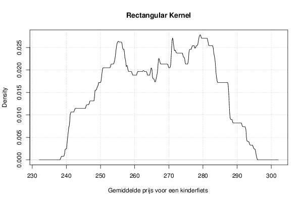
mydensity3<-density(x,bw=bw,kernel='rectangular',na.rm=TRUE)
mydensity[,3] = signif(mydensity3$y,3)
plot(mydensity3,main='Rectangular Kernel',xlab=xlab,ylab=ylab)
grid()
dev.off()
bitmap(file='density4.png')
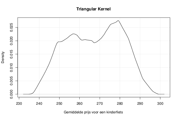
mydensity4<-density(x,bw=bw,kernel='triangular',na.rm=TRUE)
mydensity[,4] = signif(mydensity4$y,3)
plot(mydensity4,main='Triangular Kernel',xlab=xlab,ylab=ylab)
grid()
dev.off()
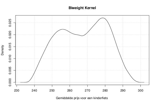
bitmap(file='density5.png')
mydensity5<-density(x,bw=bw,kernel='biweight',na.rm=TRUE)
mydensity[,5] = signif(mydensity5$y,3)
plot(mydensity5,main='Biweight Kernel',xlab=xlab,ylab=ylab)
grid()
dev.off()
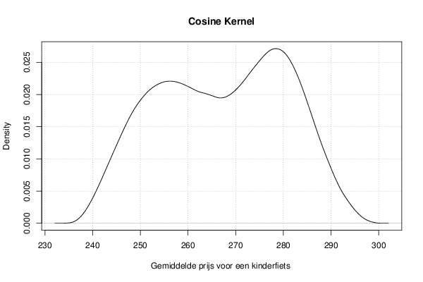
bitmap(file='density6.png')
mydensity6<-density(x,bw=bw,kernel='cosine',na.rm=TRUE)
mydensity[,6] = signif(mydensity6$y,3)
plot(mydensity6,main='Cosine Kernel',xlab=xlab,ylab=ylab)
grid()
dev.off()
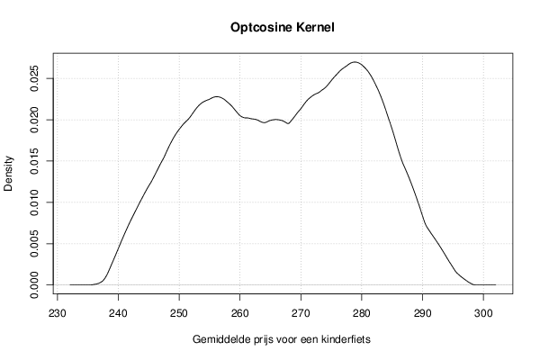
bitmap(file='density7.png')
mydensity7<-density(x,bw=bw,kernel='optcosine',na.rm=TRUE)
mydensity[,7] = signif(mydensity7$y,3)
plot(mydensity7,main='Optcosine Kernel',xlab=xlab,ylab=ylab)
grid()
dev.off()
load(file='createtable')
a<-table.start()
a<-table.row.start(a)
a<-table.element(a,'Properties of Density Trace',2,TRUE)
a<-table.row.end(a)
a<-table.row.start(a)
a<-table.element(a,'Bandwidth',header=TRUE)
a<-table.element(a,mydensity1$bw)
a<-table.row.end(a)
a<-table.row.start(a)
a<-table.element(a,'#Observations',header=TRUE)
a<-table.element(a,mydensity1$n)
a<-table.row.end(a)
a<-table.end(a)
table.save(a,file='mytable.tab')
a<-table.start()
a<-table.row.start(a)
a<-table.element(a,'Maximum Density Values',3,TRUE)
a<-table.row.end(a)
a<-table.row.start(a)
a<-table.element(a,'Kernel',1,TRUE)
a<-table.element(a,'x-value',1,TRUE)
a<-table.element(a,'max. density',1,TRUE)
a<-table.row.end(a)
a<-table.row.start(a)
a<-table.element(a,'Gaussian',1,TRUE)
a<-table.element(a,mydensity1$x[mydensity1$y==max(mydensity1$y)],1)
a<-table.element(a,mydensity1$y[mydensity1$y==max(mydensity1$y)],1)
a<-table.row.end(a)
a<-table.row.start(a)
a<-table.element(a,'Epanechnikov',1,TRUE)
a<-table.element(a,mydensity2$x[mydensity2$y==max(mydensity2$y)],1)
a<-table.element(a,mydensity2$y[mydensity2$y==max(mydensity2$y)],1)
a<-table.row.end(a)
a<-table.row.start(a)
a<-table.element(a,'Rectangular',1,TRUE)
a<-table.element(a,mydensity3$x[mydensity3$y==max(mydensity3$y)],1)
a<-table.element(a,mydensity3$y[mydensity3$y==max(mydensity3$y)],1)
a<-table.row.end(a)
a<-table.row.start(a)
a<-table.element(a,'Triangular',1,TRUE)
a<-table.element(a,mydensity4$x[mydensity4$y==max(mydensity4$y)],1)
a<-table.element(a,mydensity4$y[mydensity4$y==max(mydensity4$y)],1)
a<-table.row.end(a)
a<-table.row.start(a)
a<-table.element(a,'Biweight',1,TRUE)
a<-table.element(a,mydensity5$x[mydensity5$y==max(mydensity5$y)],1)
a<-table.element(a,mydensity5$y[mydensity5$y==max(mydensity5$y)],1)
a<-table.row.end(a)
a<-table.row.start(a)
a<-table.element(a,'Cosine',1,TRUE)
a<-table.element(a,mydensity6$x[mydensity6$y==max(mydensity6$y)],1)
a<-table.element(a,mydensity6$y[mydensity6$y==max(mydensity6$y)],1)
a<-table.row.end(a)
a<-table.row.start(a)
a<-table.element(a,'Optcosine',1,TRUE)
a<-table.element(a,mydensity7$x[mydensity7$y==max(mydensity7$y)],1)
a<-table.element(a,mydensity7$y[mydensity7$y==max(mydensity7$y)],1)
a<-table.row.end(a)
a<-table.end(a)
table.save(a,file='mytable2.tab')
if (par2=='yes') {
a<-table.start()
a<-table.row.start(a)
a<-table.element(a,'Kernel Density Values',8,TRUE)
a<-table.row.end(a)
a<-table.row.start(a)
a<-table.element(a,'x-value',1,TRUE)
a<-table.element(a,'Gaussian',1,TRUE)
a<-table.element(a,'Epanechnikov',1,TRUE)
a<-table.element(a,'Rectangular',1,TRUE)
a<-table.element(a,'Triangular',1,TRUE)
a<-table.element(a,'Biweight',1,TRUE)
a<-table.element(a,'Cosine',1,TRUE)
a<-table.element(a,'Optcosine',1,TRUE)
a<-table.row.end(a)
for(i in 1:par3) {
a<-table.row.start(a)
a<-table.element(a,mydensity[i,8],1,TRUE)
for(j in 1:7) {
a<-table.element(a,mydensity[i,j],1)
}
a<-table.row.end(a)
}
a<-table.end(a)
table.save(a,file='mytable1.tab')
}