Free Statistics

of Irreproducible Research!

Author's title

Author*Unverified author*
R Software Modulerwasp_smp.wasp
Title produced by softwareStandard Deviation-Mean Plot
Date of computationSun, 16 Aug 2015 19:58:36 +0100
Cite this page as followsStatistical Computations at FreeStatistics.org, Office for Research Development and Education, URL https://freestatistics.org/blog/index.php?v=date/2015/Aug/16/t143975181780gsrmxdvqc0dmh.htm/, Retrieved Sat, 18 May 2024 06:32:46 +0000
Statistical Computations at FreeStatistics.org, Office for Research Development and Education, URL https://freestatistics.org/blog/index.php?pk=280201, Retrieved Sat, 18 May 2024 06:32:46 +0000
QR Codes:

Original text written by user:
IsPrivate?No (this computation is public)
User-defined keywords
Estimated Impact80
Family? (F = Feedback message, R = changed R code, M = changed R Module, P = changed Parameters, D = changed Data)
-     [Variability] [] [2014-11-24 12:14:04] [46d78fa4bef23992fc20db72a2a0da97]
- RMPD  [(Partial) Autocorrelation Function] [] [2015-08-16 18:29:51] [46d78fa4bef23992fc20db72a2a0da97]
- RMP       [Standard Deviation-Mean Plot] [] [2015-08-16 18:58:36] [fced41568b3cc41e6659ad201d611503] [Current]
Feedback Forum

Post a new message
Dataseries X:
95320.00
94965.00
94605.00
93860.00
101230.00
100840.00
95320.00
91650.00
92005.00
92005.00
92400.00
93110.00
94215.00
94215.00
93505.00
91650.00
101230.00
102690.00
100485.00
95320.00
97530.00
94215.00
95710.00
96425.00
97170.00
95320.00
95710.00
93110.00
101230.00
103795.00
101590.00
97530.00
101945.00
97170.00
101590.00
101230.00
102335.00
98275.00
102690.00
102335.00
108960.00
107465.00
101590.00
98630.00
102690.00
97170.00
101230.00
101945.00
103440.00
100130.00
101945.00
103050.00
107110.00
103795.00
99380.00
94605.00
99025.00
86875.00
92755.00
96065.00
99380.00
94605.00
94605.00
94605.00
97170.00
93505.00
88695.00
84670.00
87590.00
76190.00
83175.00
87235.00
87980.00
83920.00
84275.00
83175.00
86875.00
84275.00
79150.00
75445.00
81710.00
68105.00
76940.00
80965.00
80965.00
76190.00
71775.00
71420.00
75445.00
71775.00
64795.00
59985.00
65150.00
53005.00
64045.00
69920.00
71775.00
67715.00
62585.00
66255.00
67715.00
66610.00
55565.00
50440.00
54105.00
43065.00
54465.00
58525.00
61835.00
56315.00
51150.00
54105.00
55565.00
52645.00
41605.00
36795.00
41210.00
29065.00
42315.00
50440.00


Summary of computational transaction
Raw Inputview raw input (R code)
Raw Outputview raw output of R engine
Computing time1 seconds
R Server'Gertrude Mary Cox' @ cox.wessa.net

\begin{tabular}{lllllllll}
\hline
Summary of computational transaction \tabularnewline
Raw Input & view raw input (R code)  \tabularnewline
Raw Output & view raw output of R engine  \tabularnewline
Computing time & 1 seconds \tabularnewline
R Server & 'Gertrude Mary Cox' @ cox.wessa.net \tabularnewline
\hline
\end{tabular}
%Source: https://freestatistics.org/blog/index.php?pk=280201&T=0

[TABLE]
[ROW][C]Summary of computational transaction[/C][/ROW]
[ROW][C]Raw Input[/C][C]view raw input (R code) [/C][/ROW]
[ROW][C]Raw Output[/C][C]view raw output of R engine [/C][/ROW]
[ROW][C]Computing time[/C][C]1 seconds[/C][/ROW]
[ROW][C]R Server[/C][C]'Gertrude Mary Cox' @ cox.wessa.net[/C][/ROW]
[/TABLE]
Source: https://freestatistics.org/blog/index.php?pk=280201&T=0

Globally Unique Identifier (entire table): ba.freestatistics.org/blog/index.php?pk=280201&T=0

As an alternative you can also use a QR Code:  

The GUIDs for individual cells are displayed in the table below:

Summary of computational transaction
Raw Inputview raw input (R code)
Raw Outputview raw output of R engine
Computing time1 seconds
R Server'Gertrude Mary Cox' @ cox.wessa.net


Standard Deviation-Mean Plot
SectionMeanStandard DeviationRange
194775.83333333333211.793490285839580
296432.53407.9289231811411040
398949.16666666673342.7444041558410685
4102109.5833333333420.0720741563711790
599014.58333333335632.0392150354420235
690118.756714.9030741667923190
781067.91666666675522.1819050466119875
868705.83333333337696.6804631292327960
959901.66666666678594.3761562519228710
1047753.759511.6041867050732770

\begin{tabular}{lllllllll}
\hline
Standard Deviation-Mean Plot \tabularnewline
Section & Mean & Standard Deviation & Range \tabularnewline
1 & 94775.8333333333 & 3211.79349028583 & 9580 \tabularnewline
2 & 96432.5 & 3407.92892318114 & 11040 \tabularnewline
3 & 98949.1666666667 & 3342.74440415584 & 10685 \tabularnewline
4 & 102109.583333333 & 3420.07207415637 & 11790 \tabularnewline
5 & 99014.5833333333 & 5632.03921503544 & 20235 \tabularnewline
6 & 90118.75 & 6714.90307416679 & 23190 \tabularnewline
7 & 81067.9166666667 & 5522.18190504661 & 19875 \tabularnewline
8 & 68705.8333333333 & 7696.68046312923 & 27960 \tabularnewline
9 & 59901.6666666667 & 8594.37615625192 & 28710 \tabularnewline
10 & 47753.75 & 9511.60418670507 & 32770 \tabularnewline
\hline
\end{tabular}
%Source: https://freestatistics.org/blog/index.php?pk=280201&T=1

[TABLE]
[ROW][C]Standard Deviation-Mean Plot[/C][/ROW]
[ROW][C]Section[/C][C]Mean[/C][C]Standard Deviation[/C][C]Range[/C][/ROW]
[ROW][C]1[/C][C]94775.8333333333[/C][C]3211.79349028583[/C][C]9580[/C][/ROW]
[ROW][C]2[/C][C]96432.5[/C][C]3407.92892318114[/C][C]11040[/C][/ROW]
[ROW][C]3[/C][C]98949.1666666667[/C][C]3342.74440415584[/C][C]10685[/C][/ROW]
[ROW][C]4[/C][C]102109.583333333[/C][C]3420.07207415637[/C][C]11790[/C][/ROW]
[ROW][C]5[/C][C]99014.5833333333[/C][C]5632.03921503544[/C][C]20235[/C][/ROW]
[ROW][C]6[/C][C]90118.75[/C][C]6714.90307416679[/C][C]23190[/C][/ROW]
[ROW][C]7[/C][C]81067.9166666667[/C][C]5522.18190504661[/C][C]19875[/C][/ROW]
[ROW][C]8[/C][C]68705.8333333333[/C][C]7696.68046312923[/C][C]27960[/C][/ROW]
[ROW][C]9[/C][C]59901.6666666667[/C][C]8594.37615625192[/C][C]28710[/C][/ROW]
[ROW][C]10[/C][C]47753.75[/C][C]9511.60418670507[/C][C]32770[/C][/ROW]
[/TABLE]
Source: https://freestatistics.org/blog/index.php?pk=280201&T=1

Globally Unique Identifier (entire table): ba.freestatistics.org/blog/index.php?pk=280201&T=1

As an alternative you can also use a QR Code:  

The GUIDs for individual cells are displayed in the table below:

Standard Deviation-Mean Plot
SectionMeanStandard DeviationRange
194775.83333333333211.793490285839580
296432.53407.9289231811411040
398949.16666666673342.7444041558410685
4102109.5833333333420.0720741563711790
599014.58333333335632.0392150354420235
690118.756714.9030741667923190
781067.91666666675522.1819050466119875
868705.83333333337696.6804631292327960
959901.66666666678594.3761562519228710
1047753.759511.6041867050732770


Regression: S.E.(k) = alpha + beta * Mean(k)
alpha15196.9394612756
beta-0.113151792219188
S.D.0.0185894327362386
T-STAT-6.08688784777213
p-value0.000293686871073616

\begin{tabular}{lllllllll}
\hline
Regression: S.E.(k) = alpha + beta * Mean(k) \tabularnewline
alpha & 15196.9394612756 \tabularnewline
beta & -0.113151792219188 \tabularnewline
S.D. & 0.0185894327362386 \tabularnewline
T-STAT & -6.08688784777213 \tabularnewline
p-value & 0.000293686871073616 \tabularnewline
\hline
\end{tabular}
%Source: https://freestatistics.org/blog/index.php?pk=280201&T=2

[TABLE]
[ROW][C]Regression: S.E.(k) = alpha + beta * Mean(k)[/C][/ROW]
[ROW][C]alpha[/C][C]15196.9394612756[/C][/ROW]
[ROW][C]beta[/C][C]-0.113151792219188[/C][/ROW]
[ROW][C]S.D.[/C][C]0.0185894327362386[/C][/ROW]
[ROW][C]T-STAT[/C][C]-6.08688784777213[/C][/ROW]
[ROW][C]p-value[/C][C]0.000293686871073616[/C][/ROW]
[/TABLE]
Source: https://freestatistics.org/blog/index.php?pk=280201&T=2

Globally Unique Identifier (entire table): ba.freestatistics.org/blog/index.php?pk=280201&T=2

As an alternative you can also use a QR Code:  

The GUIDs for individual cells are displayed in the table below:

Regression: S.E.(k) = alpha + beta * Mean(k)
alpha15196.9394612756
beta-0.113151792219188
S.D.0.0185894327362386
T-STAT-6.08688784777213
p-value0.000293686871073616


Regression: ln S.E.(k) = alpha + beta * ln Mean(k)
alpha24.2435553435753
beta-1.38589065989076
S.D.0.316605261909547
T-STAT-4.37734563074541
p-value0.00235715681397514
Lambda2.38589065989076

\begin{tabular}{lllllllll}
\hline
Regression: ln S.E.(k) = alpha + beta * ln Mean(k) \tabularnewline
alpha & 24.2435553435753 \tabularnewline
beta & -1.38589065989076 \tabularnewline
S.D. & 0.316605261909547 \tabularnewline
T-STAT & -4.37734563074541 \tabularnewline
p-value & 0.00235715681397514 \tabularnewline
Lambda & 2.38589065989076 \tabularnewline
\hline
\end{tabular}
%Source: https://freestatistics.org/blog/index.php?pk=280201&T=3

[TABLE]
[ROW][C]Regression: ln S.E.(k) = alpha + beta * ln Mean(k)[/C][/ROW]
[ROW][C]alpha[/C][C]24.2435553435753[/C][/ROW]
[ROW][C]beta[/C][C]-1.38589065989076[/C][/ROW]
[ROW][C]S.D.[/C][C]0.316605261909547[/C][/ROW]
[ROW][C]T-STAT[/C][C]-4.37734563074541[/C][/ROW]
[ROW][C]p-value[/C][C]0.00235715681397514[/C][/ROW]
[ROW][C]Lambda[/C][C]2.38589065989076[/C][/ROW]
[/TABLE]
Source: https://freestatistics.org/blog/index.php?pk=280201&T=3

Globally Unique Identifier (entire table): ba.freestatistics.org/blog/index.php?pk=280201&T=3

As an alternative you can also use a QR Code:  

The GUIDs for individual cells are displayed in the table below:

Regression: ln S.E.(k) = alpha + beta * ln Mean(k)
alpha24.2435553435753
beta-1.38589065989076
S.D.0.316605261909547
T-STAT-4.37734563074541
p-value0.00235715681397514
Lambda2.38589065989076


Parameters (Session):
par1 = 12 ;
Parameters (R input):
par1 = 12 ;
R code (references can be found in the software module):
par1 <- as.numeric(par1)
(n <- length(x))
(np <- floor(n / par1))
arr <- array(NA,dim=c(par1,np))
j <- 0
k <- 1
for (i in 1:(np*par1))
{
j = j + 1
arr[j,k] <- x[i]
if (j == par1) {
j = 0
k=k+1
}
}
arr
arr.mean <- array(NA,dim=np)
arr.sd <- array(NA,dim=np)
arr.range <- array(NA,dim=np)
for (j in 1:np)
{
arr.mean[j] <- mean(arr[,j],na.rm=TRUE)
arr.sd[j] <- sd(arr[,j],na.rm=TRUE)
arr.range[j] <- max(arr[,j],na.rm=TRUE) - min(arr[,j],na.rm=TRUE)
}
arr.mean
arr.sd
arr.range
(lm1 <- lm(arr.sd~arr.mean))
(lnlm1 <- lm(log(arr.sd)~log(arr.mean)))
(lm2 <- lm(arr.range~arr.mean))
bitmap(file='test1.png')
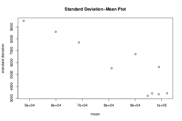
plot(arr.mean,arr.sd,main='Standard Deviation-Mean Plot',xlab='mean',ylab='standard deviation')
dev.off()
bitmap(file='test2.png')
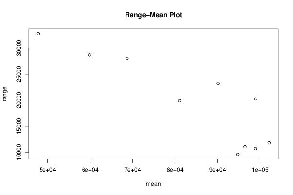
plot(arr.mean,arr.range,main='Range-Mean Plot',xlab='mean',ylab='range')
dev.off()
load(file='createtable')
a<-table.start()
a<-table.row.start(a)
a<-table.element(a,'Standard Deviation-Mean Plot',4,TRUE)
a<-table.row.end(a)
a<-table.row.start(a)
a<-table.element(a,'Section',header=TRUE)
a<-table.element(a,'Mean',header=TRUE)
a<-table.element(a,'Standard Deviation',header=TRUE)
a<-table.element(a,'Range',header=TRUE)
a<-table.row.end(a)
for (j in 1:np) {
a<-table.row.start(a)
a<-table.element(a,j,header=TRUE)
a<-table.element(a,arr.mean[j])
a<-table.element(a,arr.sd[j] )
a<-table.element(a,arr.range[j] )
a<-table.row.end(a)
}
a<-table.end(a)
table.save(a,file='mytable.tab')
a<-table.start()
a<-table.row.start(a)
a<-table.element(a,'Regression: S.E.(k) = alpha + beta * Mean(k)',2,TRUE)
a<-table.row.end(a)
a<-table.row.start(a)
a<-table.element(a,'alpha',header=TRUE)
a<-table.element(a,lm1$coefficients[[1]])
a<-table.row.end(a)
a<-table.row.start(a)
a<-table.element(a,'beta',header=TRUE)
a<-table.element(a,lm1$coefficients[[2]])
a<-table.row.end(a)
a<-table.row.start(a)
a<-table.element(a,'S.D.',header=TRUE)
a<-table.element(a,summary(lm1)$coefficients[2,2])
a<-table.row.end(a)
a<-table.row.start(a)
a<-table.element(a,'T-STAT',header=TRUE)
a<-table.element(a,summary(lm1)$coefficients[2,3])
a<-table.row.end(a)
a<-table.row.start(a)
a<-table.element(a,'p-value',header=TRUE)
a<-table.element(a,summary(lm1)$coefficients[2,4])
a<-table.row.end(a)
a<-table.end(a)
table.save(a,file='mytable1.tab')
a<-table.start()
a<-table.row.start(a)
a<-table.element(a,'Regression: ln S.E.(k) = alpha + beta * ln Mean(k)',2,TRUE)
a<-table.row.end(a)
a<-table.row.start(a)
a<-table.element(a,'alpha',header=TRUE)
a<-table.element(a,lnlm1$coefficients[[1]])
a<-table.row.end(a)
a<-table.row.start(a)
a<-table.element(a,'beta',header=TRUE)
a<-table.element(a,lnlm1$coefficients[[2]])
a<-table.row.end(a)
a<-table.row.start(a)
a<-table.element(a,'S.D.',header=TRUE)
a<-table.element(a,summary(lnlm1)$coefficients[2,2])
a<-table.row.end(a)
a<-table.row.start(a)
a<-table.element(a,'T-STAT',header=TRUE)
a<-table.element(a,summary(lnlm1)$coefficients[2,3])
a<-table.row.end(a)
a<-table.row.start(a)
a<-table.element(a,'p-value',header=TRUE)
a<-table.element(a,summary(lnlm1)$coefficients[2,4])
a<-table.row.end(a)
a<-table.row.start(a)
a<-table.element(a,'Lambda',header=TRUE)
a<-table.element(a,1-lnlm1$coefficients[[2]])
a<-table.row.end(a)
a<-table.end(a)
table.save(a,file='mytable2.tab')