Free Statistics
of Irreproducible Research!
Description of Statistical Computation | |||||||||||||||||||||
|---|---|---|---|---|---|---|---|---|---|---|---|---|---|---|---|---|---|---|---|---|---|
| Author's title | |||||||||||||||||||||
| Author | *Unverified author* | ||||||||||||||||||||
| R Software Module | rwasp_meanplot.wasp | ||||||||||||||||||||
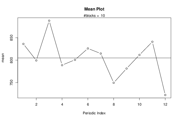
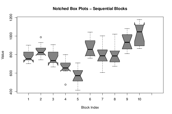
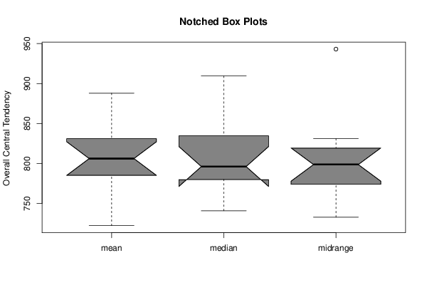
| Title produced by software | Mean Plot | ||||||||||||||||||||
| Date of computation | Fri, 27 Feb 2015 11:40:19 +0000 | ||||||||||||||||||||
| Cite this page as follows | Statistical Computations at FreeStatistics.org, Office for Research Development and Education, URL https://freestatistics.org/blog/index.php?v=date/2015/Feb/27/t1425037262d46jxgl3onyvl3f.htm/, Retrieved Sat, 18 May 2024 04:46:31 +0000 | ||||||||||||||||||||
| Statistical Computations at FreeStatistics.org, Office for Research Development and Education, URL https://freestatistics.org/blog/index.php?pk=277756, Retrieved Sat, 18 May 2024 04:46:31 +0000 | |||||||||||||||||||||
| QR Codes: | |||||||||||||||||||||
|
| |||||||||||||||||||||
| Original text written by user: | |||||||||||||||||||||
| IsPrivate? | No (this computation is public) | ||||||||||||||||||||
| User-defined keywords | |||||||||||||||||||||
| Estimated Impact | 162 | ||||||||||||||||||||
Tree of Dependent Computations | |||||||||||||||||||||
| Family? (F = Feedback message, R = changed R code, M = changed R Module, P = changed Parameters, D = changed Data) | |||||||||||||||||||||
| - [Central Tendency] [] [2015-02-27 11:22:04] [de6693ce60d0ce937e6c6e33bccc0135] - RMP [Mean Plot] [] [2015-02-27 11:40:19] [57f5dbee1b697c074ab0c7d81efd3c32] [Current] | |||||||||||||||||||||
| Feedback Forum | |||||||||||||||||||||
Post a new message | |||||||||||||||||||||
Dataset | |||||||||||||||||||||
| Dataseries X: | |||||||||||||||||||||
732 768 902 739 744 848 745 752 833 703 824 759 797 840 988 819 831 904 814 798 828 789 930 744 832 826 907 776 835 715 729 733 736 712 711 667 799 661 692 649 729 622 671 635 648 744 624 476 710 515 461 590 415 554 585 513 591 561 684 668 795 776 1043 964 762 1030 939 779 918 839 874 840 794 820 1003 780 607 1001 743 810 716 775 883 633 755 782 882 694 896 674 702 799 791 797 1021 738 1023 955 912 850 1011 872 1074 811 878 1081 956 812 1125 1051 1090 1028 1178 1041 1146 866 875 1116 903 887 | |||||||||||||||||||||
Tables (Output of Computation) | |||||||||||||||||||||
| |||||||||||||||||||||
Figures (Output of Computation) | |||||||||||||||||||||
Input Parameters & R Code | |||||||||||||||||||||
| Parameters (Session): | |||||||||||||||||||||
| par1 = 12 ; | |||||||||||||||||||||
| Parameters (R input): | |||||||||||||||||||||
| par1 = 12 ; | |||||||||||||||||||||
| R code (references can be found in the software module): | |||||||||||||||||||||
par1 <- as.numeric(par1) | |||||||||||||||||||||