Free Statistics
of Irreproducible Research!
Description of Statistical Computation | |||||||||||||||||||||||||||||||||||||||||||||||||||||||||||||||||||||||||||||||||||||||||||||||||||||||||||||||||||||||||||||||||||||||||||||||||||||||||||||||||||||||||||||||||||||||||||||||||||||||||
|---|---|---|---|---|---|---|---|---|---|---|---|---|---|---|---|---|---|---|---|---|---|---|---|---|---|---|---|---|---|---|---|---|---|---|---|---|---|---|---|---|---|---|---|---|---|---|---|---|---|---|---|---|---|---|---|---|---|---|---|---|---|---|---|---|---|---|---|---|---|---|---|---|---|---|---|---|---|---|---|---|---|---|---|---|---|---|---|---|---|---|---|---|---|---|---|---|---|---|---|---|---|---|---|---|---|---|---|---|---|---|---|---|---|---|---|---|---|---|---|---|---|---|---|---|---|---|---|---|---|---|---|---|---|---|---|---|---|---|---|---|---|---|---|---|---|---|---|---|---|---|---|---|---|---|---|---|---|---|---|---|---|---|---|---|---|---|---|---|---|---|---|---|---|---|---|---|---|---|---|---|---|---|---|---|---|---|---|---|---|---|---|---|---|---|---|---|---|---|---|---|---|
| Author's title | |||||||||||||||||||||||||||||||||||||||||||||||||||||||||||||||||||||||||||||||||||||||||||||||||||||||||||||||||||||||||||||||||||||||||||||||||||||||||||||||||||||||||||||||||||||||||||||||||||||||||
| Author | *The author of this computation has been verified* | ||||||||||||||||||||||||||||||||||||||||||||||||||||||||||||||||||||||||||||||||||||||||||||||||||||||||||||||||||||||||||||||||||||||||||||||||||||||||||||||||||||||||||||||||||||||||||||||||||||||||
| R Software Module | rwasp_histogram.wasp | ||||||||||||||||||||||||||||||||||||||||||||||||||||||||||||||||||||||||||||||||||||||||||||||||||||||||||||||||||||||||||||||||||||||||||||||||||||||||||||||||||||||||||||||||||||||||||||||||||||||||
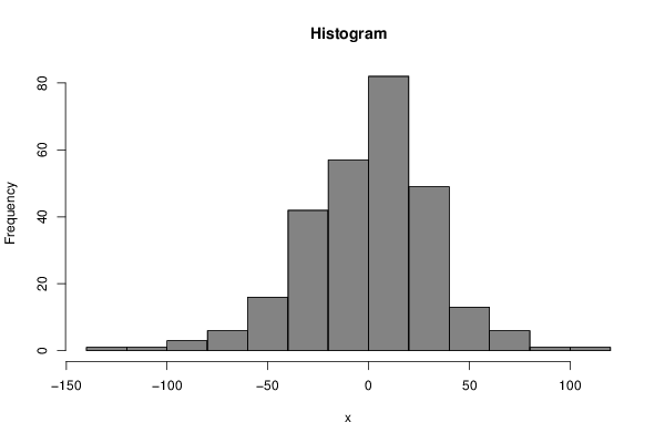
| Title produced by software | Histogram | ||||||||||||||||||||||||||||||||||||||||||||||||||||||||||||||||||||||||||||||||||||||||||||||||||||||||||||||||||||||||||||||||||||||||||||||||||||||||||||||||||||||||||||||||||||||||||||||||||||||||
| Date of computation | Tue, 20 Jan 2015 11:20:18 +0000 | ||||||||||||||||||||||||||||||||||||||||||||||||||||||||||||||||||||||||||||||||||||||||||||||||||||||||||||||||||||||||||||||||||||||||||||||||||||||||||||||||||||||||||||||||||||||||||||||||||||||||
| Cite this page as follows | Statistical Computations at FreeStatistics.org, Office for Research Development and Education, URL https://freestatistics.org/blog/index.php?v=date/2015/Jan/20/t14217528308b1utten2ziigzy.htm/, Retrieved Wed, 15 May 2024 11:32:34 +0000 | ||||||||||||||||||||||||||||||||||||||||||||||||||||||||||||||||||||||||||||||||||||||||||||||||||||||||||||||||||||||||||||||||||||||||||||||||||||||||||||||||||||||||||||||||||||||||||||||||||||||||
| Statistical Computations at FreeStatistics.org, Office for Research Development and Education, URL https://freestatistics.org/blog/index.php?pk=275082, Retrieved Wed, 15 May 2024 11:32:34 +0000 | |||||||||||||||||||||||||||||||||||||||||||||||||||||||||||||||||||||||||||||||||||||||||||||||||||||||||||||||||||||||||||||||||||||||||||||||||||||||||||||||||||||||||||||||||||||||||||||||||||||||||
| QR Codes: | |||||||||||||||||||||||||||||||||||||||||||||||||||||||||||||||||||||||||||||||||||||||||||||||||||||||||||||||||||||||||||||||||||||||||||||||||||||||||||||||||||||||||||||||||||||||||||||||||||||||||
|
| |||||||||||||||||||||||||||||||||||||||||||||||||||||||||||||||||||||||||||||||||||||||||||||||||||||||||||||||||||||||||||||||||||||||||||||||||||||||||||||||||||||||||||||||||||||||||||||||||||||||||
| Original text written by user: | |||||||||||||||||||||||||||||||||||||||||||||||||||||||||||||||||||||||||||||||||||||||||||||||||||||||||||||||||||||||||||||||||||||||||||||||||||||||||||||||||||||||||||||||||||||||||||||||||||||||||
| IsPrivate? | No (this computation is public) | ||||||||||||||||||||||||||||||||||||||||||||||||||||||||||||||||||||||||||||||||||||||||||||||||||||||||||||||||||||||||||||||||||||||||||||||||||||||||||||||||||||||||||||||||||||||||||||||||||||||||
| User-defined keywords | |||||||||||||||||||||||||||||||||||||||||||||||||||||||||||||||||||||||||||||||||||||||||||||||||||||||||||||||||||||||||||||||||||||||||||||||||||||||||||||||||||||||||||||||||||||||||||||||||||||||||
| Estimated Impact | 64 | ||||||||||||||||||||||||||||||||||||||||||||||||||||||||||||||||||||||||||||||||||||||||||||||||||||||||||||||||||||||||||||||||||||||||||||||||||||||||||||||||||||||||||||||||||||||||||||||||||||||||
Tree of Dependent Computations | |||||||||||||||||||||||||||||||||||||||||||||||||||||||||||||||||||||||||||||||||||||||||||||||||||||||||||||||||||||||||||||||||||||||||||||||||||||||||||||||||||||||||||||||||||||||||||||||||||||||||
| Family? (F = Feedback message, R = changed R code, M = changed R Module, P = changed Parameters, D = changed Data) | |||||||||||||||||||||||||||||||||||||||||||||||||||||||||||||||||||||||||||||||||||||||||||||||||||||||||||||||||||||||||||||||||||||||||||||||||||||||||||||||||||||||||||||||||||||||||||||||||||||||||
| - [Two-Way ANOVA] [proefex 4] [2015-01-20 10:22:56] [bb1b6762b7e5624d262776d3f7139d34] - RMPD [ARIMA Backward Selection] [Proefex 6] [2015-01-20 10:36:28] [bb1b6762b7e5624d262776d3f7139d34] - RMP [ARIMA Forecasting] [proefex 7] [2015-01-20 10:51:59] [bb1b6762b7e5624d262776d3f7139d34] - RM D [Multiple Regression] [proefex 8] [2015-01-20 10:59:17] [bb1b6762b7e5624d262776d3f7139d34] - RM D [Histogram] [proefex oef 10] [2015-01-20 11:20:18] [8568a324fefbb8dbb43f697bfa8d1be6] [Current] | |||||||||||||||||||||||||||||||||||||||||||||||||||||||||||||||||||||||||||||||||||||||||||||||||||||||||||||||||||||||||||||||||||||||||||||||||||||||||||||||||||||||||||||||||||||||||||||||||||||||||
| Feedback Forum | |||||||||||||||||||||||||||||||||||||||||||||||||||||||||||||||||||||||||||||||||||||||||||||||||||||||||||||||||||||||||||||||||||||||||||||||||||||||||||||||||||||||||||||||||||||||||||||||||||||||||
Post a new message | |||||||||||||||||||||||||||||||||||||||||||||||||||||||||||||||||||||||||||||||||||||||||||||||||||||||||||||||||||||||||||||||||||||||||||||||||||||||||||||||||||||||||||||||||||||||||||||||||||||||||
Dataset | |||||||||||||||||||||||||||||||||||||||||||||||||||||||||||||||||||||||||||||||||||||||||||||||||||||||||||||||||||||||||||||||||||||||||||||||||||||||||||||||||||||||||||||||||||||||||||||||||||||||||
| Dataseries X: | |||||||||||||||||||||||||||||||||||||||||||||||||||||||||||||||||||||||||||||||||||||||||||||||||||||||||||||||||||||||||||||||||||||||||||||||||||||||||||||||||||||||||||||||||||||||||||||||||||||||||
-7.34659 -3.83393 0.601079 10.1708 -19.384 76.9922 5.5307 -40.6643 7.89237 17.2903 12.6761 19.6465 -22.8607 24.2146 -102.787 -22.1468 19.5158 -27.5133 32.8225 -23.6236 9.83643 4.60699 70.5428 50.2208 -0.610172 109.513 38.3844 -17.1329 9.89147 8.93507 -50.6089 6.24831 -15.4578 17.4048 -39.2381 -41.6349 5.69034 31.4039 20.6034 4.54633 -32.8318 5.29772 18.8812 21.0418 -34.8082 32.3313 -31.5422 -6.96524 -51.1887 -19.621 16.3293 -54.3249 11.0791 51.4231 -17.4376 -28.8304 23.0113 -6.31347 -53.8408 -12.2495 13.1904 8.39642 -42.7811 59.8085 36.2483 -29.8633 38.3825 76.0114 45.9664 -1.17613 21.4147 -26.7206 -36.2753 -1.78602 -12.253 2.56265 1.16142 9.31058 -27.9482 -35.9069 -16.4696 7.28922 -19.3588 1.19328 22.2468 0.588097 -19.1513 -32.8384 -19.9199 28.5582 -27.2895 20.3171 39.2813 -9.7313 -0.942376 9.60549 18.1714 -4.9384 -7.56233 12.84 -30.4868 -3.639 -17.8985 30.4074 -5.72721 -9.3317 -5.54115 -14.7961 -55.8251 -7.45031 7.46339 3.41547 -77.9853 -70.9246 25.0086 29.244 10.2707 -13.374 60.4465 27.8033 28.7837 -65.8301 18.4629 -89.4987 -19.6233 -11.2502 9.82813 -20.7817 40.6665 -28.5946 -10.6826 26.0439 -9.82614 -7.37667 -50.715 -40.8176 -1.70087 -99.8017 14.1375 -11.3701 -11.5852 43.864 32.0648 1.17527 15.5922 5.30727 0.309518 -25.6243 0.855347 45.826 34.6051 -22.2974 25.725 38.2554 -20.4191 5.13599 36.9151 -22.4416 17.9049 -14.7084 20.6995 4.38463 35.8517 -124.977 64.3234 -31.3808 22.9819 9.22512 7.16268 -6.14016 10.5282 19.031 40.8665 38.6731 38.6731 28.9975 -6.40377 23.1366 56.324 -81.4623 -6.58429 26.0776 19.8611 5.20928 57.0213 9.45682 7.45682 12.4568 16.3065 -34.724 -27.9697 33.4926 -10.2839 22.2461 -13.1051 -18.4536 9.35706 3.31778 -9.62075 18.7282 89.7837 -23.6847 13.0052 21.7361 -3.67581 -28.9609 -76.9933 -32.6912 49.3754 17.3415 -49.6868 25.4617 -21.8287 -12.7843 14.6583 -21.7871 9.07381 48.8847 -33.9381 10.7993 13.2289 -33.8785 -23.4321 7.38082 39.5195 -41.808 9.4401 1.73577 -11.3687 14.4103 36.7927 11.4415 3.58295 42.2508 -29.7848 -79.3484 -47.2454 22.0011 -55.9352 -1.49485 -25.0235 -28.1147 15.2404 64.3234 -1.89631 29.7924 31.3961 -13.8095 -7.75536 10.6631 12.0411 -54.9164 5.60625 -11.4533 36.1205 14.2016 -21.5212 -47.5903 11.8037 25.0071 -31.3808 -9.64807 7.74461 15.2404 8.14127 -17.6636 -23.8619 22.1111 24.4277 -35.2637 25.4359 -11.1429 9.01713 12.6079 19.19 -22.1745 21.192 -67.4088 | |||||||||||||||||||||||||||||||||||||||||||||||||||||||||||||||||||||||||||||||||||||||||||||||||||||||||||||||||||||||||||||||||||||||||||||||||||||||||||||||||||||||||||||||||||||||||||||||||||||||||
Tables (Output of Computation) | |||||||||||||||||||||||||||||||||||||||||||||||||||||||||||||||||||||||||||||||||||||||||||||||||||||||||||||||||||||||||||||||||||||||||||||||||||||||||||||||||||||||||||||||||||||||||||||||||||||||||
| |||||||||||||||||||||||||||||||||||||||||||||||||||||||||||||||||||||||||||||||||||||||||||||||||||||||||||||||||||||||||||||||||||||||||||||||||||||||||||||||||||||||||||||||||||||||||||||||||||||||||
Figures (Output of Computation) | |||||||||||||||||||||||||||||||||||||||||||||||||||||||||||||||||||||||||||||||||||||||||||||||||||||||||||||||||||||||||||||||||||||||||||||||||||||||||||||||||||||||||||||||||||||||||||||||||||||||||
Input Parameters & R Code | |||||||||||||||||||||||||||||||||||||||||||||||||||||||||||||||||||||||||||||||||||||||||||||||||||||||||||||||||||||||||||||||||||||||||||||||||||||||||||||||||||||||||||||||||||||||||||||||||||||||||
| Parameters (Session): | |||||||||||||||||||||||||||||||||||||||||||||||||||||||||||||||||||||||||||||||||||||||||||||||||||||||||||||||||||||||||||||||||||||||||||||||||||||||||||||||||||||||||||||||||||||||||||||||||||||||||
| par1 = FALSE ; par2 = -0.3 ; par3 = 0 ; par4 = 1 ; par5 = 12 ; par6 = 3 ; par7 = 0 ; par8 = 2 ; par9 = 0 ; | |||||||||||||||||||||||||||||||||||||||||||||||||||||||||||||||||||||||||||||||||||||||||||||||||||||||||||||||||||||||||||||||||||||||||||||||||||||||||||||||||||||||||||||||||||||||||||||||||||||||||
| Parameters (R input): | |||||||||||||||||||||||||||||||||||||||||||||||||||||||||||||||||||||||||||||||||||||||||||||||||||||||||||||||||||||||||||||||||||||||||||||||||||||||||||||||||||||||||||||||||||||||||||||||||||||||||
| par1 = ; par2 = grey ; par3 = FALSE ; par4 = Unknown ; | |||||||||||||||||||||||||||||||||||||||||||||||||||||||||||||||||||||||||||||||||||||||||||||||||||||||||||||||||||||||||||||||||||||||||||||||||||||||||||||||||||||||||||||||||||||||||||||||||||||||||
| R code (references can be found in the software module): | |||||||||||||||||||||||||||||||||||||||||||||||||||||||||||||||||||||||||||||||||||||||||||||||||||||||||||||||||||||||||||||||||||||||||||||||||||||||||||||||||||||||||||||||||||||||||||||||||||||||||
par1 <- as.numeric(par1) | |||||||||||||||||||||||||||||||||||||||||||||||||||||||||||||||||||||||||||||||||||||||||||||||||||||||||||||||||||||||||||||||||||||||||||||||||||||||||||||||||||||||||||||||||||||||||||||||||||||||||