Free Statistics
of Irreproducible Research!
Description of Statistical Computation | |||||||||||||||||||||
|---|---|---|---|---|---|---|---|---|---|---|---|---|---|---|---|---|---|---|---|---|---|
| Author's title | |||||||||||||||||||||
| Author | *Unverified author* | ||||||||||||||||||||
| R Software Module | rwasp_meanplot.wasp | ||||||||||||||||||||
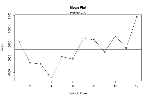
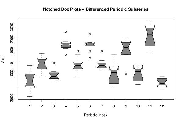
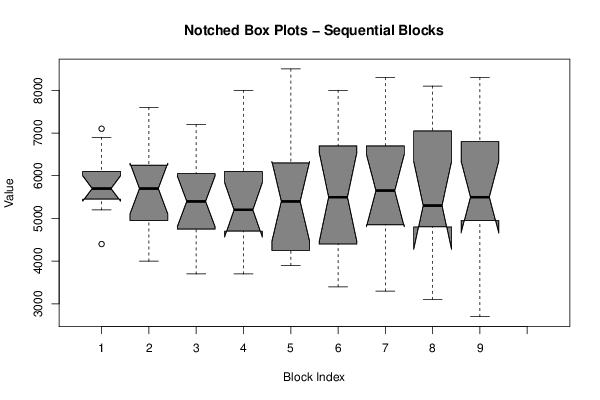
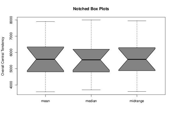
| Title produced by software | Mean Plot | ||||||||||||||||||||
| Date of computation | Mon, 08 Aug 2016 13:02:23 +0100 | ||||||||||||||||||||
| Cite this page as follows | Statistical Computations at FreeStatistics.org, Office for Research Development and Education, URL https://freestatistics.org/blog/index.php?v=date/2016/Aug/08/t1470657889t8xe7yrw5yp9pui.htm/, Retrieved Mon, 29 Apr 2024 10:45:17 +0000 | ||||||||||||||||||||
| Statistical Computations at FreeStatistics.org, Office for Research Development and Education, URL https://freestatistics.org/blog/index.php?pk=296087, Retrieved Mon, 29 Apr 2024 10:45:17 +0000 | |||||||||||||||||||||
| QR Codes: | |||||||||||||||||||||
|
| |||||||||||||||||||||
| Original text written by user: | |||||||||||||||||||||
| IsPrivate? | No (this computation is public) | ||||||||||||||||||||
| User-defined keywords | |||||||||||||||||||||
| Estimated Impact | 153 | ||||||||||||||||||||
Tree of Dependent Computations | |||||||||||||||||||||
| Family? (F = Feedback message, R = changed R code, M = changed R Module, P = changed Parameters, D = changed Data) | |||||||||||||||||||||
| - [Mean Plot] [] [2015-10-16 14:42:22] [39c526a439265efa15f7db403b90ebd6] - R PD [Mean Plot] [] [2016-08-08 12:02:23] [047b71d569822bc9ea0d1a14ab5e311b] [Current] | |||||||||||||||||||||
| Feedback Forum | |||||||||||||||||||||
Post a new message | |||||||||||||||||||||
Dataset | |||||||||||||||||||||
| Dataseries X: | |||||||||||||||||||||
5400 5200 5500 4400 5700 5600 6000 6200 6900 6000 5700 7100 6000 4500 5300 4000 5600 4600 6100 5500 5800 6500 6400 7600 5500 4600 5100 3700 5300 4100 5800 5500 4900 7000 6300 7200 5400 5000 4500 3700 4900 4400 6000 5800 5000 6700 6200 8000 6400 3900 3900 3900 4600 4600 6200 5700 5100 6400 5900 8500 6700 3900 4100 3400 4700 5400 6800 6700 5400 6300 5600 8000 6100 4900 4400 3300 4900 5900 6900 6500 4800 6900 5400 8300 6900 5000 4600 3100 4900 4700 7100 7100 5400 7000 5200 8100 6900 5100 3900 2700 5300 5100 6700 7700 5700 6400 4800 8300 | |||||||||||||||||||||
Tables (Output of Computation) | |||||||||||||||||||||
| |||||||||||||||||||||
Figures (Output of Computation) | |||||||||||||||||||||
Input Parameters & R Code | |||||||||||||||||||||
| Parameters (Session): | |||||||||||||||||||||
| par1 = 0.01 ; par2 = 0.99 ; par3 = 0.01 ; | |||||||||||||||||||||
| Parameters (R input): | |||||||||||||||||||||
| par1 = 12 ; | |||||||||||||||||||||
| R code (references can be found in the software module): | |||||||||||||||||||||
par1 <- as.numeric(par1) | |||||||||||||||||||||