Free Statistics
of Irreproducible Research!
Description of Statistical Computation | |||||||||||||||||||||
|---|---|---|---|---|---|---|---|---|---|---|---|---|---|---|---|---|---|---|---|---|---|
| Author's title | |||||||||||||||||||||
| Author | *Unverified author* | ||||||||||||||||||||
| R Software Module | rwasp_meanplot.wasp | ||||||||||||||||||||
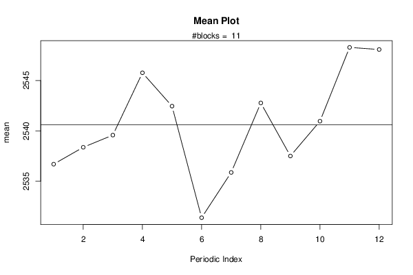
| Title produced by software | Mean Plot | ||||||||||||||||||||
| Date of computation | Mon, 08 Aug 2016 23:33:02 +0100 | ||||||||||||||||||||
| Cite this page as follows | Statistical Computations at FreeStatistics.org, Office for Research Development and Education, URL https://freestatistics.org/blog/index.php?v=date/2016/Aug/08/t1470695625ll3wsp8sxobj8xe.htm/, Retrieved Mon, 29 Apr 2024 08:33:43 +0000 | ||||||||||||||||||||
| Statistical Computations at FreeStatistics.org, Office for Research Development and Education, URL https://freestatistics.org/blog/index.php?pk=296107, Retrieved Mon, 29 Apr 2024 08:33:43 +0000 | |||||||||||||||||||||
| QR Codes: | |||||||||||||||||||||
|
| |||||||||||||||||||||
| Original text written by user: | |||||||||||||||||||||
| IsPrivate? | No (this computation is public) | ||||||||||||||||||||
| User-defined keywords | |||||||||||||||||||||
| Estimated Impact | 157 | ||||||||||||||||||||
Tree of Dependent Computations | |||||||||||||||||||||
| Family? (F = Feedback message, R = changed R code, M = changed R Module, P = changed Parameters, D = changed Data) | |||||||||||||||||||||
| - [Univariate Data Series] [omzet lego technique] [2016-08-08 19:25:41] [74be16979710d4c4e7c6647856088456] - RMPD [Harrell-Davis Quantiles] [Harrel-Davis quan...] [2016-08-08 22:07:37] [4c392b130fccc63297597dd6ffb6df17] - RM [Mean Plot] [mean plot lego te...] [2016-08-08 22:33:02] [d7adcc7732e5b057da1b42af54844e1a] [Current] | |||||||||||||||||||||
| Feedback Forum | |||||||||||||||||||||
Post a new message | |||||||||||||||||||||
Dataset | |||||||||||||||||||||
| Dataseries X: | |||||||||||||||||||||
2443.6 2460.2 2448.2 2470.4 2484.7 2466.8 2487.9 2508.4 2510.5 2497.4 2532.5 2556.8 2561 2547.3 2541.5 2558.5 2587.9 2580.5 2579.6 2589.3 2595 2595.6 2588.8 2591.7 2601.7 2585.4 2573.3 2597.4 2600.6 2570.6 2569.4 2584.9 2608.8 2617.2 2621 2540.5 2554.5 2601.9 2623 2640.7 2640.7 2619.8 2624.2 2638.2 2645.7 2679.6 2669 2664.6 2663.3 2667.4 2653.2 2630.8 2626.6 2641.9 2625.8 2606 2594.4 2583.6 2588.7 2600.3 2579.5 2576.6 2597.8 2595.6 2599 2621.7 2645.6 2644.2 2625.6 2624.6 2596.2 2599.5 2584.1 2570.8 2555 2574.5 2576.7 2579 2588.7 2601.1 2575.7 2559.5 2561.1 2528.3 2514.7 2558.5 2553.3 2577.1 2566 2549.5 2527.8 2540.9 2534.2 2538 2559 2554.9 2575.5 2546.5 2561.6 2546.6 2502.9 2463.1 2472.6 2463.5 2446.3 2456.2 2471.5 2447.5 2428.6 2420.2 2414.9 2420.2 2423.8 2407 2388.7 2409.6 2392 2380.2 2423.3 2451.6 2440.8 2432.9 2413.6 2391.6 2358.1 2345.4 2384.4 2384.4 2384.4 2418.7 2420 2493.1 2493.1 2492.8 | |||||||||||||||||||||
Tables (Output of Computation) | |||||||||||||||||||||
| |||||||||||||||||||||
Figures (Output of Computation) | |||||||||||||||||||||
Input Parameters & R Code | |||||||||||||||||||||
| Parameters (Session): | |||||||||||||||||||||
| Parameters (R input): | |||||||||||||||||||||
| par1 = 12 ; | |||||||||||||||||||||
| R code (references can be found in the software module): | |||||||||||||||||||||
par1 <- as.numeric(par1) | |||||||||||||||||||||