Repository of Reproducible Computations

Free Statistics

of Irreproducible Research!

Author's title

Author

*Unverified author*

R Software Module

rwasp_autocorrelation.wasp

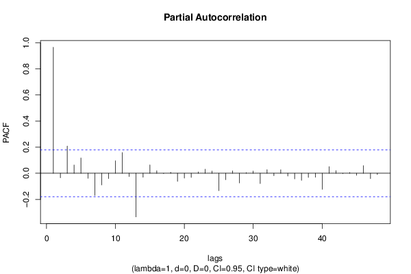
Title produced by software

(Partial) Autocorrelation Function

Date of computation

Wed, 10 Aug 2016 14:53:09 +0100

Cite this page as follows

Statistical Computations at FreeStatistics.org, Office for Research Development and Education, URL https://freestatistics.org/blog/index.php?v=date/2016/Aug/10/t1470837293b0x37d9j6d4ylel.htm/, Retrieved Tue, 30 Apr 2024 03:39:57 +0000

Statistical Computations at FreeStatistics.org, Office for Research Development and Education, URL https://freestatistics.org/blog/index.php?pk=296203, Retrieved Tue, 30 Apr 2024 03:39:57 +0000

QR Codes:

Paste this QR Code to cite your computation.

Original text written by user:

IsPrivate?

No (this computation is public)

User-defined keywords

Estimated Impact

112

Family? (F = Feedback message, R = changed R code, M = changed R Module, P = changed Parameters, D = changed Data)

-       [(Partial) Autocorrelation Function] [Braadoven Omzet -...] [2016-08-10 13:53:09] [d41d8cd98f00b204e9800998ecf8427e] [Current]
- R P     [(Partial) Autocorrelation Function] [Braadoven Omzet -...] [2016-08-10 14:12:55] [74be16979710d4c4e7c6647856088456] 
- RMP     [Standard Deviation Plot] [Braadoven Omzet -...] [2016-08-10 16:11:10] [74be16979710d4c4e7c6647856088456] 
- RMP     [Standard Deviation-Mean Plot] [Braadoven Omzet -...] [2016-08-10 22:00:44] [74be16979710d4c4e7c6647856088456] 
- RMP     [Classical Decomposition] [Braadoven Omzet -...] [2016-08-10 22:37:09] [74be16979710d4c4e7c6647856088456] 
- RMPD    [Univariate Data Series] [Nagasaki Bomb Mus...] [2016-08-10 23:12:55] [74be16979710d4c4e7c6647856088456] 
- RMPD    [Histogram] [Nagasaki Bomb Mus...] [2016-08-10 23:18:05] [74be16979710d4c4e7c6647856088456] 
- RMPD    [Kernel Density Estimation] [Nagasaki Bomb Mus...] [2016-08-10 23:28:52] [74be16979710d4c4e7c6647856088456] 
- RMPD    [Notched Boxplots] [Nagasaki Bomb Mus...] [2016-08-10 23:36:27] [74be16979710d4c4e7c6647856088456] 

Feedback Forum

Post a new message

Dataseries X:

Download CSV

Histogram

Boxplots

Summary of computational transaction
Raw Input	view raw input (R code)
Raw Output	view raw output of R engine
Computing time	1 seconds
R Server	'Sir Maurice George Kendall' @ kendall.wessa.net

\begin{tabular}{lllllllll}
\hline
Summary of computational transaction \tabularnewline
Raw Input & view raw input (R code)  \tabularnewline
Raw Output & view raw output of R engine  \tabularnewline
Computing time & 1 seconds \tabularnewline
R Server & 'Sir Maurice George Kendall' @ kendall.wessa.net \tabularnewline
\hline
\end{tabular}
%Source: https://freestatistics.org/blog/index.php?pk=296203&T=0

[TABLE]
[ROW][C]Summary of computational transaction[/C][/ROW]
[ROW][C]Raw Input[/C][C]view raw input (R code) [/C][/ROW]
[ROW][C]Raw Output[/C][C]view raw output of R engine [/C][/ROW]
[ROW][C]Computing time[/C][C]1 seconds[/C][/ROW]
[ROW][C]R Server[/C][C]'Sir Maurice George Kendall' @ kendall.wessa.net[/C][/ROW]
[/TABLE]
Source: https://freestatistics.org/blog/index.php?pk=296203&T=0

Globally Unique Identifier (entire table): ba.freestatistics.org/blog/index.php?pk=296203&T=0

As an alternative you can also use a QR Code:

The GUIDs for individual cells are displayed in the table below:

Summary of computational transaction
Raw Input	view raw input (R code)
Raw Output	view raw output of R engine
Computing time	1 seconds
R Server	'Sir Maurice George Kendall' @ kendall.wessa.net

Autocorrelation Function
Time lag k	ACF(k)	T-STAT	P-value
1	0.966416	10.5866	0
2	0.931664	10.2059	0
3	0.911827	9.9886	0
4	0.89732	9.8297	0
5	0.887642	9.7236	0
6	0.8738	9.572	0
7	0.846519	9.2732	0
8	0.815094	8.9289	0
9	0.787612	8.6279	0
10	0.770882	8.4446	0
11	0.765646	8.3872	0
12	0.754209	8.2619	0
13	0.7158	7.8412	0
14	0.676715	7.413	0
15	0.65122	7.1338	0
16	0.632168	6.9251	0
17	0.616302	6.7512	0
18	0.597814	6.5487	0
19	0.56695	6.2106	0
20	0.531612	5.8235	0
21	0.500931	5.4874	0
22	0.480796	5.2669	0
23	0.469309	5.141	1e-06
24	0.452553	4.9575	1e-06
25	0.415318	4.5496	6e-06
26	0.376306	4.1222	3.5e-05
27	0.349467	3.8282	0.000103
28	0.325372	3.5643	0.000262
29	0.305218	3.3435	0.000552
30	0.284924	3.1212	0.001128
31	0.250774	2.7471	0.00347
32	0.215135	2.3567	0.010029
33	0.185301	2.0299	0.022291
34	0.165622	1.8143	0.036065
35	0.152	1.6651	0.049253
36	0.131167	1.4369	0.07668
37	0.095612	1.0474	0.148516
38	0.059587	0.6527	0.257584
39	0.031897	0.3494	0.363695
40	0.003854	0.0422	0.483198
41	-0.016649	-0.1824	0.427795
42	-0.03591	-0.3934	0.347369
43	-0.06643	-0.7277	0.234107
44	-0.098184	-1.0756	0.142142
45	-0.123797	-1.3561	0.088802
46	-0.13845	-1.5166	0.065993
47	-0.149949	-1.6426	0.051541
48	-0.167092	-1.8304	0.034836

\begin{tabular}{lllllllll}
\hline
Autocorrelation Function \tabularnewline
Time lag k & ACF(k) & T-STAT & P-value \tabularnewline
1 & 0.966416 & 10.5866 & 0 \tabularnewline
2 & 0.931664 & 10.2059 & 0 \tabularnewline
3 & 0.911827 & 9.9886 & 0 \tabularnewline
4 & 0.89732 & 9.8297 & 0 \tabularnewline
5 & 0.887642 & 9.7236 & 0 \tabularnewline
6 & 0.8738 & 9.572 & 0 \tabularnewline
7 & 0.846519 & 9.2732 & 0 \tabularnewline
8 & 0.815094 & 8.9289 & 0 \tabularnewline
9 & 0.787612 & 8.6279 & 0 \tabularnewline
10 & 0.770882 & 8.4446 & 0 \tabularnewline
11 & 0.765646 & 8.3872 & 0 \tabularnewline
12 & 0.754209 & 8.2619 & 0 \tabularnewline
13 & 0.7158 & 7.8412 & 0 \tabularnewline
14 & 0.676715 & 7.413 & 0 \tabularnewline
15 & 0.65122 & 7.1338 & 0 \tabularnewline
16 & 0.632168 & 6.9251 & 0 \tabularnewline
17 & 0.616302 & 6.7512 & 0 \tabularnewline
18 & 0.597814 & 6.5487 & 0 \tabularnewline
19 & 0.56695 & 6.2106 & 0 \tabularnewline
20 & 0.531612 & 5.8235 & 0 \tabularnewline
21 & 0.500931 & 5.4874 & 0 \tabularnewline
22 & 0.480796 & 5.2669 & 0 \tabularnewline
23 & 0.469309 & 5.141 & 1e-06 \tabularnewline
24 & 0.452553 & 4.9575 & 1e-06 \tabularnewline
25 & 0.415318 & 4.5496 & 6e-06 \tabularnewline
26 & 0.376306 & 4.1222 & 3.5e-05 \tabularnewline
27 & 0.349467 & 3.8282 & 0.000103 \tabularnewline
28 & 0.325372 & 3.5643 & 0.000262 \tabularnewline
29 & 0.305218 & 3.3435 & 0.000552 \tabularnewline
30 & 0.284924 & 3.1212 & 0.001128 \tabularnewline
31 & 0.250774 & 2.7471 & 0.00347 \tabularnewline
32 & 0.215135 & 2.3567 & 0.010029 \tabularnewline
33 & 0.185301 & 2.0299 & 0.022291 \tabularnewline
34 & 0.165622 & 1.8143 & 0.036065 \tabularnewline
35 & 0.152 & 1.6651 & 0.049253 \tabularnewline
36 & 0.131167 & 1.4369 & 0.07668 \tabularnewline
37 & 0.095612 & 1.0474 & 0.148516 \tabularnewline
38 & 0.059587 & 0.6527 & 0.257584 \tabularnewline
39 & 0.031897 & 0.3494 & 0.363695 \tabularnewline
40 & 0.003854 & 0.0422 & 0.483198 \tabularnewline
41 & -0.016649 & -0.1824 & 0.427795 \tabularnewline
42 & -0.03591 & -0.3934 & 0.347369 \tabularnewline
43 & -0.06643 & -0.7277 & 0.234107 \tabularnewline
44 & -0.098184 & -1.0756 & 0.142142 \tabularnewline
45 & -0.123797 & -1.3561 & 0.088802 \tabularnewline
46 & -0.13845 & -1.5166 & 0.065993 \tabularnewline
47 & -0.149949 & -1.6426 & 0.051541 \tabularnewline
48 & -0.167092 & -1.8304 & 0.034836 \tabularnewline
\hline
\end{tabular}
%Source: https://freestatistics.org/blog/index.php?pk=296203&T=1

[TABLE]
[ROW][C]Autocorrelation Function[/C][/ROW]
[ROW][C]Time lag k[/C][C]ACF(k)[/C][C]T-STAT[/C][C]P-value[/C][/ROW]
[ROW][C]1[/C][C]0.966416[/C][C]10.5866[/C][C]0[/C][/ROW]
[ROW][C]2[/C][C]0.931664[/C][C]10.2059[/C][C]0[/C][/ROW]
[ROW][C]3[/C][C]0.911827[/C][C]9.9886[/C][C]0[/C][/ROW]
[ROW][C]4[/C][C]0.89732[/C][C]9.8297[/C][C]0[/C][/ROW]
[ROW][C]5[/C][C]0.887642[/C][C]9.7236[/C][C]0[/C][/ROW]
[ROW][C]6[/C][C]0.8738[/C][C]9.572[/C][C]0[/C][/ROW]
[ROW][C]7[/C][C]0.846519[/C][C]9.2732[/C][C]0[/C][/ROW]
[ROW][C]8[/C][C]0.815094[/C][C]8.9289[/C][C]0[/C][/ROW]
[ROW][C]9[/C][C]0.787612[/C][C]8.6279[/C][C]0[/C][/ROW]
[ROW][C]10[/C][C]0.770882[/C][C]8.4446[/C][C]0[/C][/ROW]
[ROW][C]11[/C][C]0.765646[/C][C]8.3872[/C][C]0[/C][/ROW]
[ROW][C]12[/C][C]0.754209[/C][C]8.2619[/C][C]0[/C][/ROW]
[ROW][C]13[/C][C]0.7158[/C][C]7.8412[/C][C]0[/C][/ROW]
[ROW][C]14[/C][C]0.676715[/C][C]7.413[/C][C]0[/C][/ROW]
[ROW][C]15[/C][C]0.65122[/C][C]7.1338[/C][C]0[/C][/ROW]
[ROW][C]16[/C][C]0.632168[/C][C]6.9251[/C][C]0[/C][/ROW]
[ROW][C]17[/C][C]0.616302[/C][C]6.7512[/C][C]0[/C][/ROW]
[ROW][C]18[/C][C]0.597814[/C][C]6.5487[/C][C]0[/C][/ROW]
[ROW][C]19[/C][C]0.56695[/C][C]6.2106[/C][C]0[/C][/ROW]
[ROW][C]20[/C][C]0.531612[/C][C]5.8235[/C][C]0[/C][/ROW]
[ROW][C]21[/C][C]0.500931[/C][C]5.4874[/C][C]0[/C][/ROW]
[ROW][C]22[/C][C]0.480796[/C][C]5.2669[/C][C]0[/C][/ROW]
[ROW][C]23[/C][C]0.469309[/C][C]5.141[/C][C]1e-06[/C][/ROW]
[ROW][C]24[/C][C]0.452553[/C][C]4.9575[/C][C]1e-06[/C][/ROW]
[ROW][C]25[/C][C]0.415318[/C][C]4.5496[/C][C]6e-06[/C][/ROW]
[ROW][C]26[/C][C]0.376306[/C][C]4.1222[/C][C]3.5e-05[/C][/ROW]
[ROW][C]27[/C][C]0.349467[/C][C]3.8282[/C][C]0.000103[/C][/ROW]
[ROW][C]28[/C][C]0.325372[/C][C]3.5643[/C][C]0.000262[/C][/ROW]
[ROW][C]29[/C][C]0.305218[/C][C]3.3435[/C][C]0.000552[/C][/ROW]
[ROW][C]30[/C][C]0.284924[/C][C]3.1212[/C][C]0.001128[/C][/ROW]
[ROW][C]31[/C][C]0.250774[/C][C]2.7471[/C][C]0.00347[/C][/ROW]
[ROW][C]32[/C][C]0.215135[/C][C]2.3567[/C][C]0.010029[/C][/ROW]
[ROW][C]33[/C][C]0.185301[/C][C]2.0299[/C][C]0.022291[/C][/ROW]
[ROW][C]34[/C][C]0.165622[/C][C]1.8143[/C][C]0.036065[/C][/ROW]
[ROW][C]35[/C][C]0.152[/C][C]1.6651[/C][C]0.049253[/C][/ROW]
[ROW][C]36[/C][C]0.131167[/C][C]1.4369[/C][C]0.07668[/C][/ROW]
[ROW][C]37[/C][C]0.095612[/C][C]1.0474[/C][C]0.148516[/C][/ROW]
[ROW][C]38[/C][C]0.059587[/C][C]0.6527[/C][C]0.257584[/C][/ROW]
[ROW][C]39[/C][C]0.031897[/C][C]0.3494[/C][C]0.363695[/C][/ROW]
[ROW][C]40[/C][C]0.003854[/C][C]0.0422[/C][C]0.483198[/C][/ROW]
[ROW][C]41[/C][C]-0.016649[/C][C]-0.1824[/C][C]0.427795[/C][/ROW]
[ROW][C]42[/C][C]-0.03591[/C][C]-0.3934[/C][C]0.347369[/C][/ROW]
[ROW][C]43[/C][C]-0.06643[/C][C]-0.7277[/C][C]0.234107[/C][/ROW]
[ROW][C]44[/C][C]-0.098184[/C][C]-1.0756[/C][C]0.142142[/C][/ROW]
[ROW][C]45[/C][C]-0.123797[/C][C]-1.3561[/C][C]0.088802[/C][/ROW]
[ROW][C]46[/C][C]-0.13845[/C][C]-1.5166[/C][C]0.065993[/C][/ROW]
[ROW][C]47[/C][C]-0.149949[/C][C]-1.6426[/C][C]0.051541[/C][/ROW]
[ROW][C]48[/C][C]-0.167092[/C][C]-1.8304[/C][C]0.034836[/C][/ROW]
[/TABLE]
Source: https://freestatistics.org/blog/index.php?pk=296203&T=1

Globally Unique Identifier (entire table): ba.freestatistics.org/blog/index.php?pk=296203&T=1

As an alternative you can also use a QR Code:

The GUIDs for individual cells are displayed in the table below:

Autocorrelation Function
Time lag k	ACF(k)	T-STAT	P-value
1	0.966416	10.5866	0
2	0.931664	10.2059	0
3	0.911827	9.9886	0
4	0.89732	9.8297	0
5	0.887642	9.7236	0
6	0.8738	9.572	0
7	0.846519	9.2732	0
8	0.815094	8.9289	0
9	0.787612	8.6279	0
10	0.770882	8.4446	0
11	0.765646	8.3872	0
12	0.754209	8.2619	0
13	0.7158	7.8412	0
14	0.676715	7.413	0
15	0.65122	7.1338	0
16	0.632168	6.9251	0
17	0.616302	6.7512	0
18	0.597814	6.5487	0
19	0.56695	6.2106	0
20	0.531612	5.8235	0
21	0.500931	5.4874	0
22	0.480796	5.2669	0
23	0.469309	5.141	1e-06
24	0.452553	4.9575	1e-06
25	0.415318	4.5496	6e-06
26	0.376306	4.1222	3.5e-05
27	0.349467	3.8282	0.000103
28	0.325372	3.5643	0.000262
29	0.305218	3.3435	0.000552
30	0.284924	3.1212	0.001128
31	0.250774	2.7471	0.00347
32	0.215135	2.3567	0.010029
33	0.185301	2.0299	0.022291
34	0.165622	1.8143	0.036065
35	0.152	1.6651	0.049253
36	0.131167	1.4369	0.07668
37	0.095612	1.0474	0.148516
38	0.059587	0.6527	0.257584
39	0.031897	0.3494	0.363695
40	0.003854	0.0422	0.483198
41	-0.016649	-0.1824	0.427795
42	-0.03591	-0.3934	0.347369
43	-0.06643	-0.7277	0.234107
44	-0.098184	-1.0756	0.142142
45	-0.123797	-1.3561	0.088802
46	-0.13845	-1.5166	0.065993
47	-0.149949	-1.6426	0.051541
48	-0.167092	-1.8304	0.034836

Partial Autocorrelation Function
Time lag k	PACF(k)	T-STAT	P-value
1	0.966416	10.5866	0
2	-0.034755	-0.3807	0.352041
3	0.208419	2.2831	0.012092
4	0.063766	0.6985	0.243101
5	0.11739	1.2859	0.100469
6	-0.037903	-0.4152	0.339367
7	-0.169762	-1.8597	0.032692
8	-0.089849	-0.9842	0.163488
9	-0.040236	-0.4408	0.330089
10	0.096084	1.0525	0.147332
11	0.158377	1.7349	0.042661
12	-0.025335	-0.2775	0.390923
13	-0.334452	-3.6637	0.000186
14	-0.030766	-0.337	0.368343
15	0.064342	0.7048	0.241141
16	0.019979	0.2189	0.413566
17	-0.002378	-0.026	0.489632
18	0.007741	0.0848	0.46628
19	-0.062073	-0.68	0.248916
20	-0.037211	-0.4076	0.342137
21	-0.031934	-0.3498	0.363542
22	0.010412	0.1141	0.454691
23	0.031309	0.343	0.36611
24	0.016603	0.1819	0.427994
25	-0.133458	-1.462	0.073184
26	-0.049394	-0.5411	0.294725
27	0.018728	0.2051	0.418901
28	-0.074218	-0.813	0.208908
29	0.005435	0.0595	0.476313
30	0.017238	0.1888	0.425272
31	-0.079185	-0.8674	0.19372
32	0.027799	0.3045	0.380628
33	-0.018737	-0.2053	0.41886
34	0.026987	0.2956	0.384013
35	-0.021646	-0.2371	0.406486
36	-0.042848	-0.4694	0.319825
37	-0.054524	-0.5973	0.275721
38	-0.031963	-0.3501	0.363423
39	-0.03021	-0.3309	0.370636
40	-0.122955	-1.3469	0.090275
41	0.051234	0.5612	0.287842
42	0.020082	0.22	0.413128
43	-0.002535	-0.0278	0.488946
44	0.005902	0.0647	0.47428
45	-0.01546	-0.1694	0.4329
46	0.058257	0.6382	0.262289
47	-0.04055	-0.4442	0.32885
48	-0.009774	-0.1071	0.457456

\begin{tabular}{lllllllll}
\hline
Partial Autocorrelation Function \tabularnewline
Time lag k & PACF(k) & T-STAT & P-value \tabularnewline
1 & 0.966416 & 10.5866 & 0 \tabularnewline
2 & -0.034755 & -0.3807 & 0.352041 \tabularnewline
3 & 0.208419 & 2.2831 & 0.012092 \tabularnewline
4 & 0.063766 & 0.6985 & 0.243101 \tabularnewline
5 & 0.11739 & 1.2859 & 0.100469 \tabularnewline
6 & -0.037903 & -0.4152 & 0.339367 \tabularnewline
7 & -0.169762 & -1.8597 & 0.032692 \tabularnewline
8 & -0.089849 & -0.9842 & 0.163488 \tabularnewline
9 & -0.040236 & -0.4408 & 0.330089 \tabularnewline
10 & 0.096084 & 1.0525 & 0.147332 \tabularnewline
11 & 0.158377 & 1.7349 & 0.042661 \tabularnewline
12 & -0.025335 & -0.2775 & 0.390923 \tabularnewline
13 & -0.334452 & -3.6637 & 0.000186 \tabularnewline
14 & -0.030766 & -0.337 & 0.368343 \tabularnewline
15 & 0.064342 & 0.7048 & 0.241141 \tabularnewline
16 & 0.019979 & 0.2189 & 0.413566 \tabularnewline
17 & -0.002378 & -0.026 & 0.489632 \tabularnewline
18 & 0.007741 & 0.0848 & 0.46628 \tabularnewline
19 & -0.062073 & -0.68 & 0.248916 \tabularnewline
20 & -0.037211 & -0.4076 & 0.342137 \tabularnewline
21 & -0.031934 & -0.3498 & 0.363542 \tabularnewline
22 & 0.010412 & 0.1141 & 0.454691 \tabularnewline
23 & 0.031309 & 0.343 & 0.36611 \tabularnewline
24 & 0.016603 & 0.1819 & 0.427994 \tabularnewline
25 & -0.133458 & -1.462 & 0.073184 \tabularnewline
26 & -0.049394 & -0.5411 & 0.294725 \tabularnewline
27 & 0.018728 & 0.2051 & 0.418901 \tabularnewline
28 & -0.074218 & -0.813 & 0.208908 \tabularnewline
29 & 0.005435 & 0.0595 & 0.476313 \tabularnewline
30 & 0.017238 & 0.1888 & 0.425272 \tabularnewline
31 & -0.079185 & -0.8674 & 0.19372 \tabularnewline
32 & 0.027799 & 0.3045 & 0.380628 \tabularnewline
33 & -0.018737 & -0.2053 & 0.41886 \tabularnewline
34 & 0.026987 & 0.2956 & 0.384013 \tabularnewline
35 & -0.021646 & -0.2371 & 0.406486 \tabularnewline
36 & -0.042848 & -0.4694 & 0.319825 \tabularnewline
37 & -0.054524 & -0.5973 & 0.275721 \tabularnewline
38 & -0.031963 & -0.3501 & 0.363423 \tabularnewline
39 & -0.03021 & -0.3309 & 0.370636 \tabularnewline
40 & -0.122955 & -1.3469 & 0.090275 \tabularnewline
41 & 0.051234 & 0.5612 & 0.287842 \tabularnewline
42 & 0.020082 & 0.22 & 0.413128 \tabularnewline
43 & -0.002535 & -0.0278 & 0.488946 \tabularnewline
44 & 0.005902 & 0.0647 & 0.47428 \tabularnewline
45 & -0.01546 & -0.1694 & 0.4329 \tabularnewline
46 & 0.058257 & 0.6382 & 0.262289 \tabularnewline
47 & -0.04055 & -0.4442 & 0.32885 \tabularnewline
48 & -0.009774 & -0.1071 & 0.457456 \tabularnewline
\hline
\end{tabular}
%Source: https://freestatistics.org/blog/index.php?pk=296203&T=2

[TABLE]
[ROW][C]Partial Autocorrelation Function[/C][/ROW]
[ROW][C]Time lag k[/C][C]PACF(k)[/C][C]T-STAT[/C][C]P-value[/C][/ROW]
[ROW][C]1[/C][C]0.966416[/C][C]10.5866[/C][C]0[/C][/ROW]
[ROW][C]2[/C][C]-0.034755[/C][C]-0.3807[/C][C]0.352041[/C][/ROW]
[ROW][C]3[/C][C]0.208419[/C][C]2.2831[/C][C]0.012092[/C][/ROW]
[ROW][C]4[/C][C]0.063766[/C][C]0.6985[/C][C]0.243101[/C][/ROW]
[ROW][C]5[/C][C]0.11739[/C][C]1.2859[/C][C]0.100469[/C][/ROW]
[ROW][C]6[/C][C]-0.037903[/C][C]-0.4152[/C][C]0.339367[/C][/ROW]
[ROW][C]7[/C][C]-0.169762[/C][C]-1.8597[/C][C]0.032692[/C][/ROW]
[ROW][C]8[/C][C]-0.089849[/C][C]-0.9842[/C][C]0.163488[/C][/ROW]
[ROW][C]9[/C][C]-0.040236[/C][C]-0.4408[/C][C]0.330089[/C][/ROW]
[ROW][C]10[/C][C]0.096084[/C][C]1.0525[/C][C]0.147332[/C][/ROW]
[ROW][C]11[/C][C]0.158377[/C][C]1.7349[/C][C]0.042661[/C][/ROW]
[ROW][C]12[/C][C]-0.025335[/C][C]-0.2775[/C][C]0.390923[/C][/ROW]
[ROW][C]13[/C][C]-0.334452[/C][C]-3.6637[/C][C]0.000186[/C][/ROW]
[ROW][C]14[/C][C]-0.030766[/C][C]-0.337[/C][C]0.368343[/C][/ROW]
[ROW][C]15[/C][C]0.064342[/C][C]0.7048[/C][C]0.241141[/C][/ROW]
[ROW][C]16[/C][C]0.019979[/C][C]0.2189[/C][C]0.413566[/C][/ROW]
[ROW][C]17[/C][C]-0.002378[/C][C]-0.026[/C][C]0.489632[/C][/ROW]
[ROW][C]18[/C][C]0.007741[/C][C]0.0848[/C][C]0.46628[/C][/ROW]
[ROW][C]19[/C][C]-0.062073[/C][C]-0.68[/C][C]0.248916[/C][/ROW]
[ROW][C]20[/C][C]-0.037211[/C][C]-0.4076[/C][C]0.342137[/C][/ROW]
[ROW][C]21[/C][C]-0.031934[/C][C]-0.3498[/C][C]0.363542[/C][/ROW]
[ROW][C]22[/C][C]0.010412[/C][C]0.1141[/C][C]0.454691[/C][/ROW]
[ROW][C]23[/C][C]0.031309[/C][C]0.343[/C][C]0.36611[/C][/ROW]
[ROW][C]24[/C][C]0.016603[/C][C]0.1819[/C][C]0.427994[/C][/ROW]
[ROW][C]25[/C][C]-0.133458[/C][C]-1.462[/C][C]0.073184[/C][/ROW]
[ROW][C]26[/C][C]-0.049394[/C][C]-0.5411[/C][C]0.294725[/C][/ROW]
[ROW][C]27[/C][C]0.018728[/C][C]0.2051[/C][C]0.418901[/C][/ROW]
[ROW][C]28[/C][C]-0.074218[/C][C]-0.813[/C][C]0.208908[/C][/ROW]
[ROW][C]29[/C][C]0.005435[/C][C]0.0595[/C][C]0.476313[/C][/ROW]
[ROW][C]30[/C][C]0.017238[/C][C]0.1888[/C][C]0.425272[/C][/ROW]
[ROW][C]31[/C][C]-0.079185[/C][C]-0.8674[/C][C]0.19372[/C][/ROW]
[ROW][C]32[/C][C]0.027799[/C][C]0.3045[/C][C]0.380628[/C][/ROW]
[ROW][C]33[/C][C]-0.018737[/C][C]-0.2053[/C][C]0.41886[/C][/ROW]
[ROW][C]34[/C][C]0.026987[/C][C]0.2956[/C][C]0.384013[/C][/ROW]
[ROW][C]35[/C][C]-0.021646[/C][C]-0.2371[/C][C]0.406486[/C][/ROW]
[ROW][C]36[/C][C]-0.042848[/C][C]-0.4694[/C][C]0.319825[/C][/ROW]
[ROW][C]37[/C][C]-0.054524[/C][C]-0.5973[/C][C]0.275721[/C][/ROW]
[ROW][C]38[/C][C]-0.031963[/C][C]-0.3501[/C][C]0.363423[/C][/ROW]
[ROW][C]39[/C][C]-0.03021[/C][C]-0.3309[/C][C]0.370636[/C][/ROW]
[ROW][C]40[/C][C]-0.122955[/C][C]-1.3469[/C][C]0.090275[/C][/ROW]
[ROW][C]41[/C][C]0.051234[/C][C]0.5612[/C][C]0.287842[/C][/ROW]
[ROW][C]42[/C][C]0.020082[/C][C]0.22[/C][C]0.413128[/C][/ROW]
[ROW][C]43[/C][C]-0.002535[/C][C]-0.0278[/C][C]0.488946[/C][/ROW]
[ROW][C]44[/C][C]0.005902[/C][C]0.0647[/C][C]0.47428[/C][/ROW]
[ROW][C]45[/C][C]-0.01546[/C][C]-0.1694[/C][C]0.4329[/C][/ROW]
[ROW][C]46[/C][C]0.058257[/C][C]0.6382[/C][C]0.262289[/C][/ROW]
[ROW][C]47[/C][C]-0.04055[/C][C]-0.4442[/C][C]0.32885[/C][/ROW]
[ROW][C]48[/C][C]-0.009774[/C][C]-0.1071[/C][C]0.457456[/C][/ROW]
[/TABLE]
Source: https://freestatistics.org/blog/index.php?pk=296203&T=2

Globally Unique Identifier (entire table): ba.freestatistics.org/blog/index.php?pk=296203&T=2

As an alternative you can also use a QR Code:

The GUIDs for individual cells are displayed in the table below:

Partial Autocorrelation Function
Time lag k	PACF(k)	T-STAT	P-value
1	0.966416	10.5866	0
2	-0.034755	-0.3807	0.352041
3	0.208419	2.2831	0.012092
4	0.063766	0.6985	0.243101
5	0.11739	1.2859	0.100469
6	-0.037903	-0.4152	0.339367
7	-0.169762	-1.8597	0.032692
8	-0.089849	-0.9842	0.163488
9	-0.040236	-0.4408	0.330089
10	0.096084	1.0525	0.147332
11	0.158377	1.7349	0.042661
12	-0.025335	-0.2775	0.390923
13	-0.334452	-3.6637	0.000186
14	-0.030766	-0.337	0.368343
15	0.064342	0.7048	0.241141
16	0.019979	0.2189	0.413566
17	-0.002378	-0.026	0.489632
18	0.007741	0.0848	0.46628
19	-0.062073	-0.68	0.248916
20	-0.037211	-0.4076	0.342137
21	-0.031934	-0.3498	0.363542
22	0.010412	0.1141	0.454691
23	0.031309	0.343	0.36611
24	0.016603	0.1819	0.427994
25	-0.133458	-1.462	0.073184
26	-0.049394	-0.5411	0.294725
27	0.018728	0.2051	0.418901
28	-0.074218	-0.813	0.208908
29	0.005435	0.0595	0.476313
30	0.017238	0.1888	0.425272
31	-0.079185	-0.8674	0.19372
32	0.027799	0.3045	0.380628
33	-0.018737	-0.2053	0.41886
34	0.026987	0.2956	0.384013
35	-0.021646	-0.2371	0.406486
36	-0.042848	-0.4694	0.319825
37	-0.054524	-0.5973	0.275721
38	-0.031963	-0.3501	0.363423
39	-0.03021	-0.3309	0.370636
40	-0.122955	-1.3469	0.090275
41	0.051234	0.5612	0.287842
42	0.020082	0.22	0.413128
43	-0.002535	-0.0278	0.488946
44	0.005902	0.0647	0.47428
45	-0.01546	-0.1694	0.4329
46	0.058257	0.6382	0.262289
47	-0.04055	-0.4442	0.32885
48	-0.009774	-0.1071	0.457456

Figure 1

PNG link

Postscript link

PDF link

Figure 2

PNG link

Postscript link

PDF link

Figure 3

PNG link

Postscript link

PDF link

Parameters (Session):

par1 = 48 ; par2 = 1 ; par3 = 0 ; par4 = 0 ; par5 = 12 ; par6 = White Noise ; par7 = 0.95 ;

Parameters (R input):

par1 = 48 ; par2 = 1 ; par3 = 0 ; par4 = 0 ; par5 = 12 ; par6 = White Noise ; par7 = 0.95 ; par8 = ;

R code (references can be found in the software module):

par8 <- ''
par7 <- '0.95'
par6 <- 'White Noise'
par5 <- '12'
par4 <- '0'
par3 <- '0'
par2 <- '1'
par1 <- 'Default'
if (par1 == 'Default') {
par1 = 10*log10(length(x))
} else {
par1 <- as.numeric(par1)
}
par2 <- as.numeric(par2)
par3 <- as.numeric(par3)
par4 <- as.numeric(par4)
par5 <- as.numeric(par5)
if (par6 == 'White Noise') par6 <- 'white' else par6 <- 'ma'
par7 <- as.numeric(par7)
if (par8 != '') par8 <- as.numeric(par8)
x <- na.omit(x)
ox <- x
if (par8 == '') {
if (par2 == 0) {
x <- log(x)
} else {
x <- (x ^ par2 - 1) / par2
}
} else {
x <- log(x,base=par8)
}
if (par3 > 0) x <- diff(x,lag=1,difference=par3)
if (par4 > 0) x <- diff(x,lag=par5,difference=par4)
bitmap(file='picts.png')
op <- par(mfrow=c(2,1))
plot(ox,type='l',main='Original Time Series',xlab='time',ylab='value')
if (par8=='') {
mytitle <- paste('Working Time Series (lambda=',par2,', d=',par3,', D=',par4,')',sep='')
mysub <- paste('(lambda=',par2,', d=',par3,', D=',par4,', CI=', par7, ', CI type=',par6,')',sep='')
} else {
mytitle <- paste('Working Time Series (base=',par8,', d=',par3,', D=',par4,')',sep='')
mysub <- paste('(base=',par8,', d=',par3,', D=',par4,', CI=', par7, ', CI type=',par6,')',sep='')
}
plot(x,type='l', main=mytitle,xlab='time',ylab='value')
par(op)
dev.off()
bitmap(file='pic1.png')
racf <- acf(x, par1, main='Autocorrelation', xlab='time lag', ylab='ACF', ci.type=par6, ci=par7, sub=mysub)
dev.off()
bitmap(file='pic2.png')
rpacf <- pacf(x,par1,main='Partial Autocorrelation',xlab='lags',ylab='PACF',sub=mysub)
dev.off()
(myacf <- c(racf$acf))
(mypacf <- c(rpacf$acf))
lengthx <- length(x)
sqrtn <- sqrt(lengthx)
load(file='createtable')
a<-table.start()
a<-table.row.start(a)
a<-table.element(a,'Autocorrelation Function',4,TRUE)
a<-table.row.end(a)
a<-table.row.start(a)
a<-table.element(a,'Time lag k',header=TRUE)
a<-table.element(a,hyperlink('basics.htm','ACF(k)','click here for more information about the Autocorrelation Function'),header=TRUE)
a<-table.element(a,'T-STAT',header=TRUE)
a<-table.element(a,'P-value',header=TRUE)
a<-table.row.end(a)
for (i in 2:(par1+1)) {
a<-table.row.start(a)
a<-table.element(a,i-1,header=TRUE)
a<-table.element(a,round(myacf[i],6))
mytstat <- myacf[i]*sqrtn
a<-table.element(a,round(mytstat,4))
a<-table.element(a,round(1-pt(abs(mytstat),lengthx),6))
a<-table.row.end(a)
}
a<-table.end(a)
table.save(a,file='mytable.tab')
a<-table.start()
a<-table.row.start(a)
a<-table.element(a,'Partial Autocorrelation Function',4,TRUE)
a<-table.row.end(a)
a<-table.row.start(a)
a<-table.element(a,'Time lag k',header=TRUE)
a<-table.element(a,hyperlink('basics.htm','PACF(k)','click here for more information about the Partial Autocorrelation Function'),header=TRUE)
a<-table.element(a,'T-STAT',header=TRUE)
a<-table.element(a,'P-value',header=TRUE)
a<-table.row.end(a)
for (i in 1:par1) {
a<-table.row.start(a)
a<-table.element(a,i,header=TRUE)
a<-table.element(a,round(mypacf[i],6))
mytstat <- mypacf[i]*sqrtn
a<-table.element(a,round(mytstat,4))
a<-table.element(a,round(1-pt(abs(mytstat),lengthx),6))
a<-table.row.end(a)
}
a<-table.end(a)
table.save(a,file='mytable1.tab')

Free Statistics

Description of Statistical Computation

Tree of Dependent Computations

Dataset

Tables (Output of Computation)

Figures (Output of Computation)

Input Parameters & R Code