Free Statistics
of Irreproducible Research!
Description of Statistical Computation | |||||||||||||||||||||
|---|---|---|---|---|---|---|---|---|---|---|---|---|---|---|---|---|---|---|---|---|---|
| Author's title | |||||||||||||||||||||
| Author | *Unverified author* | ||||||||||||||||||||
| R Software Module | rwasp_meanplot.wasp | ||||||||||||||||||||
| Title produced by software | Mean Plot | ||||||||||||||||||||
| Date of computation | Thu, 11 Aug 2016 16:01:26 +0100 | ||||||||||||||||||||
| Cite this page as follows | Statistical Computations at FreeStatistics.org, Office for Research Development and Education, URL https://freestatistics.org/blog/index.php?v=date/2016/Aug/11/t14709277138slf96myuyn24g1.htm/, Retrieved Sun, 05 May 2024 20:20:49 +0000 | ||||||||||||||||||||
| Statistical Computations at FreeStatistics.org, Office for Research Development and Education, URL https://freestatistics.org/blog/index.php?pk=296322, Retrieved Sun, 05 May 2024 20:20:49 +0000 | |||||||||||||||||||||
| QR Codes: | |||||||||||||||||||||
|
| |||||||||||||||||||||
| Original text written by user: | |||||||||||||||||||||
| IsPrivate? | No (this computation is public) | ||||||||||||||||||||
| User-defined keywords | |||||||||||||||||||||
| Estimated Impact | 107 | ||||||||||||||||||||
Tree of Dependent Computations | |||||||||||||||||||||
| Family? (F = Feedback message, R = changed R code, M = changed R Module, P = changed Parameters, D = changed Data) | |||||||||||||||||||||
| - [Mean Plot] [Reeks A stap 17] [2016-08-11 15:01:26] [efea2b8bc7c91838390b884e612c3e3f] [Current] - R D [Mean Plot] [mean plot lego te...] [2016-08-12 00:34:45] [4c392b130fccc63297597dd6ffb6df17] | |||||||||||||||||||||
| Feedback Forum | |||||||||||||||||||||
Post a new message | |||||||||||||||||||||
Dataset | |||||||||||||||||||||
| Dataseries X: | |||||||||||||||||||||
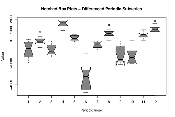
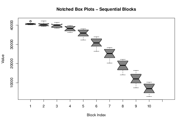
40927.00 40856.00 40778.00 40635.00 42103.00 42032.00 40927.00 40194.00 40265.00 40265.00 40336.00 40486.00 40856.00 40414.00 40856.00 40486.00 41661.00 42181.00 39973.00 39381.00 39894.00 39823.00 39381.00 39453.00 40336.00 40194.00 40336.00 40336.00 41298.00 41440.00 38790.00 38790.00 39823.00 39310.00 38427.00 38790.00 39674.00 39232.00 39161.00 38206.00 39602.00 39894.00 37023.00 36952.00 38427.00 37615.00 36218.00 36810.00 37465.00 37615.00 37173.00 36290.00 38128.00 38128.00 34893.00 34673.00 35556.00 33939.00 32314.00 32835.00 33939.00 33055.00 32464.00 31210.00 32906.00 32977.00 29743.00 29664.00 30256.00 28418.00 26430.00 27235.00 28339.00 27164.00 27093.00 25910.00 27826.00 28197.00 24585.00 23780.00 24293.00 22305.00 20246.00 20909.00 22156.00 20688.00 20909.00 20026.00 21864.00 22084.00 17668.00 17375.00 18180.00 16050.00 14134.00 14797.00 16414.00 14504.00 14355.00 12880.00 14504.00 15017.00 10451.00 10451.00 11113.00 9347.00 7359.00 8392.00 10230.00 8242.00 9055.00 7950.00 9717.00 10308.00 5592.00 5229.00 5963.00 4196.00 2800.00 3384.00 | |||||||||||||||||||||
Tables (Output of Computation) | |||||||||||||||||||||
| |||||||||||||||||||||
Figures (Output of Computation) | |||||||||||||||||||||
Input Parameters & R Code | |||||||||||||||||||||
| Parameters (Session): | |||||||||||||||||||||
| par1 = 12 ; | |||||||||||||||||||||
| Parameters (R input): | |||||||||||||||||||||
| par1 = 12 ; | |||||||||||||||||||||
| R code (references can be found in the software module): | |||||||||||||||||||||
par1 <- as.numeric(par1) | |||||||||||||||||||||