Repository of Reproducible Computations

Free Statistics

of Irreproducible Research!

Author's title

Author

*Unverified author*

R Software Module

rwasp_autocorrelation.wasp

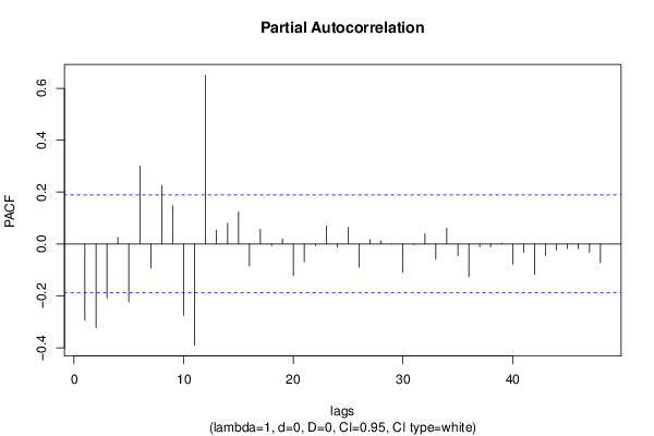
Title produced by software

(Partial) Autocorrelation Function

Date of computation

Thu, 11 Aug 2016 23:42:14 +0100

Cite this page as follows

Statistical Computations at FreeStatistics.org, Office for Research Development and Education, URL https://freestatistics.org/blog/index.php?v=date/2016/Aug/11/t14709553935yijksjjxq1gzcx.htm/, Retrieved Sun, 05 May 2024 13:17:18 +0000

Statistical Computations at FreeStatistics.org, Office for Research Development and Education, URL https://freestatistics.org/blog/index.php?pk=296384, Retrieved Sun, 05 May 2024 13:17:18 +0000

QR Codes:

Paste this QR Code to cite your computation.

Original text written by user:

IsPrivate?

No (this computation is public)

User-defined keywords

Estimated Impact

119

Family? (F = Feedback message, R = changed R code, M = changed R Module, P = changed Parameters, D = changed Data)

-     [Mean versus Median] [mean vs median va...] [2016-08-11 11:22:45] [4c392b130fccc63297597dd6ffb6df17]
- RMP   [Mean Plot] [mean en meadian p...] [2016-08-11 22:10:26] [4c392b130fccc63297597dd6ffb6df17]
- RMP       [(Partial) Autocorrelation Function] [autocorrelation a...] [2016-08-11 22:42:14] [d7adcc7732e5b057da1b42af54844e1a] [Current]
- RMP         [Classical Decomposition] [additief decompos...] [2016-08-13 11:15:14] [4c392b130fccc63297597dd6ffb6df17] 
- RMP         [Exponential Smoothing] [exponential smoot...] [2016-08-13 11:29:39] [4c392b130fccc63297597dd6ffb6df17] 
- RMPD        [Classical Decomposition] [additive decompos...] [2016-08-13 11:36:43] [4c392b130fccc63297597dd6ffb6df17] 
- RMPD        [Exponential Smoothing] [exponentional smo...] [2016-08-13 11:45:34] [4c392b130fccc63297597dd6ffb6df17] 

Feedback Forum

Post a new message

Dataseries X:

Download CSV

Histogram

Boxplots

Summary of computational transaction
Raw Input	view raw input (R code)
Raw Output	view raw output of R engine
Computing time	1 seconds
R Server	'Gertrude Mary Cox' @ cox.wessa.net

\begin{tabular}{lllllllll}
\hline
Summary of computational transaction \tabularnewline
Raw Input & view raw input (R code)  \tabularnewline
Raw Output & view raw output of R engine  \tabularnewline
Computing time & 1 seconds \tabularnewline
R Server & 'Gertrude Mary Cox' @ cox.wessa.net \tabularnewline
\hline
\end{tabular}
%Source: https://freestatistics.org/blog/index.php?pk=296384&T=0

[TABLE]
[ROW][C]Summary of computational transaction[/C][/ROW]
[ROW][C]Raw Input[/C][C]view raw input (R code) [/C][/ROW]
[ROW][C]Raw Output[/C][C]view raw output of R engine [/C][/ROW]
[ROW][C]Computing time[/C][C]1 seconds[/C][/ROW]
[ROW][C]R Server[/C][C]'Gertrude Mary Cox' @ cox.wessa.net[/C][/ROW]
[/TABLE]
Source: https://freestatistics.org/blog/index.php?pk=296384&T=0

Globally Unique Identifier (entire table): ba.freestatistics.org/blog/index.php?pk=296384&T=0

As an alternative you can also use a QR Code:

The GUIDs for individual cells are displayed in the table below:

Summary of computational transaction
Raw Input	view raw input (R code)
Raw Output	view raw output of R engine
Computing time	1 seconds
R Server	'Gertrude Mary Cox' @ cox.wessa.net

Autocorrelation Function
Time lag k	ACF(k)	T-STAT	P-value
1	-0.293325	-3.0483	0.001447
2	-0.20905	-2.1725	0.016002
3	0.005984	0.0622	0.475264
4	0.162402	1.6877	0.047174
5	-0.215887	-2.2436	0.01345
6	0.327875	3.4074	0.000461
7	-0.198963	-2.0677	0.02053
8	0.101471	1.0545	0.147
9	0.021678	0.2253	0.411092
10	-0.189682	-1.9712	0.025628
11	-0.273759	-2.845	0.002657
12	0.823069	8.5536	0
13	-0.256763	-2.6684	0.004398
14	-0.199805	-2.0764	0.020114
15	0.027986	0.2908	0.385866
16	0.147188	1.5296	0.064517
17	-0.205893	-2.1397	0.017315
18	0.312937	3.2521	0.000764
19	-0.166502	-1.7303	0.043213
20	0.015986	0.1661	0.434183
21	0.040334	0.4192	0.337965
22	-0.1497	-1.5557	0.06135
23	-0.219216	-2.2782	0.012343
24	0.653189	6.7881	0
25	-0.205995	-2.1408	0.017271
26	-0.227438	-2.3636	0.009943
27	0.067083	0.6971	0.243605
28	0.125579	1.3051	0.097324
29	-0.182989	-1.9017	0.029939
30	0.248509	2.5826	0.005572
31	-0.106575	-1.1076	0.135257
32	-0.032252	-0.3352	0.369072
33	0.041272	0.4289	0.334423
34	-0.114013	-1.1849	0.119337
35	-0.181003	-1.881	0.03133
36	0.490474	5.0972	1e-06
37	-0.149704	-1.5558	0.061345
38	-0.235519	-2.4476	0.007997
39	0.094277	0.9798	0.164698
40	0.082605	0.8585	0.19627
41	-0.155438	-1.6154	0.054576
42	0.160966	1.6728	0.048629
43	-0.047348	-0.4921	0.31184
44	-0.07719	-0.8022	0.212104
45	0.056209	0.5841	0.28017
46	-0.085211	-0.8855	0.188917
47	-0.149592	-1.5546	0.061483
48	0.338485	3.5176	0.000319

\begin{tabular}{lllllllll}
\hline
Autocorrelation Function \tabularnewline
Time lag k & ACF(k) & T-STAT & P-value \tabularnewline
1 & -0.293325 & -3.0483 & 0.001447 \tabularnewline
2 & -0.20905 & -2.1725 & 0.016002 \tabularnewline
3 & 0.005984 & 0.0622 & 0.475264 \tabularnewline
4 & 0.162402 & 1.6877 & 0.047174 \tabularnewline
5 & -0.215887 & -2.2436 & 0.01345 \tabularnewline
6 & 0.327875 & 3.4074 & 0.000461 \tabularnewline
7 & -0.198963 & -2.0677 & 0.02053 \tabularnewline
8 & 0.101471 & 1.0545 & 0.147 \tabularnewline
9 & 0.021678 & 0.2253 & 0.411092 \tabularnewline
10 & -0.189682 & -1.9712 & 0.025628 \tabularnewline
11 & -0.273759 & -2.845 & 0.002657 \tabularnewline
12 & 0.823069 & 8.5536 & 0 \tabularnewline
13 & -0.256763 & -2.6684 & 0.004398 \tabularnewline
14 & -0.199805 & -2.0764 & 0.020114 \tabularnewline
15 & 0.027986 & 0.2908 & 0.385866 \tabularnewline
16 & 0.147188 & 1.5296 & 0.064517 \tabularnewline
17 & -0.205893 & -2.1397 & 0.017315 \tabularnewline
18 & 0.312937 & 3.2521 & 0.000764 \tabularnewline
19 & -0.166502 & -1.7303 & 0.043213 \tabularnewline
20 & 0.015986 & 0.1661 & 0.434183 \tabularnewline
21 & 0.040334 & 0.4192 & 0.337965 \tabularnewline
22 & -0.1497 & -1.5557 & 0.06135 \tabularnewline
23 & -0.219216 & -2.2782 & 0.012343 \tabularnewline
24 & 0.653189 & 6.7881 & 0 \tabularnewline
25 & -0.205995 & -2.1408 & 0.017271 \tabularnewline
26 & -0.227438 & -2.3636 & 0.009943 \tabularnewline
27 & 0.067083 & 0.6971 & 0.243605 \tabularnewline
28 & 0.125579 & 1.3051 & 0.097324 \tabularnewline
29 & -0.182989 & -1.9017 & 0.029939 \tabularnewline
30 & 0.248509 & 2.5826 & 0.005572 \tabularnewline
31 & -0.106575 & -1.1076 & 0.135257 \tabularnewline
32 & -0.032252 & -0.3352 & 0.369072 \tabularnewline
33 & 0.041272 & 0.4289 & 0.334423 \tabularnewline
34 & -0.114013 & -1.1849 & 0.119337 \tabularnewline
35 & -0.181003 & -1.881 & 0.03133 \tabularnewline
36 & 0.490474 & 5.0972 & 1e-06 \tabularnewline
37 & -0.149704 & -1.5558 & 0.061345 \tabularnewline
38 & -0.235519 & -2.4476 & 0.007997 \tabularnewline
39 & 0.094277 & 0.9798 & 0.164698 \tabularnewline
40 & 0.082605 & 0.8585 & 0.19627 \tabularnewline
41 & -0.155438 & -1.6154 & 0.054576 \tabularnewline
42 & 0.160966 & 1.6728 & 0.048629 \tabularnewline
43 & -0.047348 & -0.4921 & 0.31184 \tabularnewline
44 & -0.07719 & -0.8022 & 0.212104 \tabularnewline
45 & 0.056209 & 0.5841 & 0.28017 \tabularnewline
46 & -0.085211 & -0.8855 & 0.188917 \tabularnewline
47 & -0.149592 & -1.5546 & 0.061483 \tabularnewline
48 & 0.338485 & 3.5176 & 0.000319 \tabularnewline
\hline
\end{tabular}
%Source: https://freestatistics.org/blog/index.php?pk=296384&T=1

[TABLE]
[ROW][C]Autocorrelation Function[/C][/ROW]
[ROW][C]Time lag k[/C][C]ACF(k)[/C][C]T-STAT[/C][C]P-value[/C][/ROW]
[ROW][C]1[/C][C]-0.293325[/C][C]-3.0483[/C][C]0.001447[/C][/ROW]
[ROW][C]2[/C][C]-0.20905[/C][C]-2.1725[/C][C]0.016002[/C][/ROW]
[ROW][C]3[/C][C]0.005984[/C][C]0.0622[/C][C]0.475264[/C][/ROW]
[ROW][C]4[/C][C]0.162402[/C][C]1.6877[/C][C]0.047174[/C][/ROW]
[ROW][C]5[/C][C]-0.215887[/C][C]-2.2436[/C][C]0.01345[/C][/ROW]
[ROW][C]6[/C][C]0.327875[/C][C]3.4074[/C][C]0.000461[/C][/ROW]
[ROW][C]7[/C][C]-0.198963[/C][C]-2.0677[/C][C]0.02053[/C][/ROW]
[ROW][C]8[/C][C]0.101471[/C][C]1.0545[/C][C]0.147[/C][/ROW]
[ROW][C]9[/C][C]0.021678[/C][C]0.2253[/C][C]0.411092[/C][/ROW]
[ROW][C]10[/C][C]-0.189682[/C][C]-1.9712[/C][C]0.025628[/C][/ROW]
[ROW][C]11[/C][C]-0.273759[/C][C]-2.845[/C][C]0.002657[/C][/ROW]
[ROW][C]12[/C][C]0.823069[/C][C]8.5536[/C][C]0[/C][/ROW]
[ROW][C]13[/C][C]-0.256763[/C][C]-2.6684[/C][C]0.004398[/C][/ROW]
[ROW][C]14[/C][C]-0.199805[/C][C]-2.0764[/C][C]0.020114[/C][/ROW]
[ROW][C]15[/C][C]0.027986[/C][C]0.2908[/C][C]0.385866[/C][/ROW]
[ROW][C]16[/C][C]0.147188[/C][C]1.5296[/C][C]0.064517[/C][/ROW]
[ROW][C]17[/C][C]-0.205893[/C][C]-2.1397[/C][C]0.017315[/C][/ROW]
[ROW][C]18[/C][C]0.312937[/C][C]3.2521[/C][C]0.000764[/C][/ROW]
[ROW][C]19[/C][C]-0.166502[/C][C]-1.7303[/C][C]0.043213[/C][/ROW]
[ROW][C]20[/C][C]0.015986[/C][C]0.1661[/C][C]0.434183[/C][/ROW]
[ROW][C]21[/C][C]0.040334[/C][C]0.4192[/C][C]0.337965[/C][/ROW]
[ROW][C]22[/C][C]-0.1497[/C][C]-1.5557[/C][C]0.06135[/C][/ROW]
[ROW][C]23[/C][C]-0.219216[/C][C]-2.2782[/C][C]0.012343[/C][/ROW]
[ROW][C]24[/C][C]0.653189[/C][C]6.7881[/C][C]0[/C][/ROW]
[ROW][C]25[/C][C]-0.205995[/C][C]-2.1408[/C][C]0.017271[/C][/ROW]
[ROW][C]26[/C][C]-0.227438[/C][C]-2.3636[/C][C]0.009943[/C][/ROW]
[ROW][C]27[/C][C]0.067083[/C][C]0.6971[/C][C]0.243605[/C][/ROW]
[ROW][C]28[/C][C]0.125579[/C][C]1.3051[/C][C]0.097324[/C][/ROW]
[ROW][C]29[/C][C]-0.182989[/C][C]-1.9017[/C][C]0.029939[/C][/ROW]
[ROW][C]30[/C][C]0.248509[/C][C]2.5826[/C][C]0.005572[/C][/ROW]
[ROW][C]31[/C][C]-0.106575[/C][C]-1.1076[/C][C]0.135257[/C][/ROW]
[ROW][C]32[/C][C]-0.032252[/C][C]-0.3352[/C][C]0.369072[/C][/ROW]
[ROW][C]33[/C][C]0.041272[/C][C]0.4289[/C][C]0.334423[/C][/ROW]
[ROW][C]34[/C][C]-0.114013[/C][C]-1.1849[/C][C]0.119337[/C][/ROW]
[ROW][C]35[/C][C]-0.181003[/C][C]-1.881[/C][C]0.03133[/C][/ROW]
[ROW][C]36[/C][C]0.490474[/C][C]5.0972[/C][C]1e-06[/C][/ROW]
[ROW][C]37[/C][C]-0.149704[/C][C]-1.5558[/C][C]0.061345[/C][/ROW]
[ROW][C]38[/C][C]-0.235519[/C][C]-2.4476[/C][C]0.007997[/C][/ROW]
[ROW][C]39[/C][C]0.094277[/C][C]0.9798[/C][C]0.164698[/C][/ROW]
[ROW][C]40[/C][C]0.082605[/C][C]0.8585[/C][C]0.19627[/C][/ROW]
[ROW][C]41[/C][C]-0.155438[/C][C]-1.6154[/C][C]0.054576[/C][/ROW]
[ROW][C]42[/C][C]0.160966[/C][C]1.6728[/C][C]0.048629[/C][/ROW]
[ROW][C]43[/C][C]-0.047348[/C][C]-0.4921[/C][C]0.31184[/C][/ROW]
[ROW][C]44[/C][C]-0.07719[/C][C]-0.8022[/C][C]0.212104[/C][/ROW]
[ROW][C]45[/C][C]0.056209[/C][C]0.5841[/C][C]0.28017[/C][/ROW]
[ROW][C]46[/C][C]-0.085211[/C][C]-0.8855[/C][C]0.188917[/C][/ROW]
[ROW][C]47[/C][C]-0.149592[/C][C]-1.5546[/C][C]0.061483[/C][/ROW]
[ROW][C]48[/C][C]0.338485[/C][C]3.5176[/C][C]0.000319[/C][/ROW]
[/TABLE]
Source: https://freestatistics.org/blog/index.php?pk=296384&T=1

Globally Unique Identifier (entire table): ba.freestatistics.org/blog/index.php?pk=296384&T=1

As an alternative you can also use a QR Code:

The GUIDs for individual cells are displayed in the table below:

Autocorrelation Function
Time lag k	ACF(k)	T-STAT	P-value
1	-0.293325	-3.0483	0.001447
2	-0.20905	-2.1725	0.016002
3	0.005984	0.0622	0.475264
4	0.162402	1.6877	0.047174
5	-0.215887	-2.2436	0.01345
6	0.327875	3.4074	0.000461
7	-0.198963	-2.0677	0.02053
8	0.101471	1.0545	0.147
9	0.021678	0.2253	0.411092
10	-0.189682	-1.9712	0.025628
11	-0.273759	-2.845	0.002657
12	0.823069	8.5536	0
13	-0.256763	-2.6684	0.004398
14	-0.199805	-2.0764	0.020114
15	0.027986	0.2908	0.385866
16	0.147188	1.5296	0.064517
17	-0.205893	-2.1397	0.017315
18	0.312937	3.2521	0.000764
19	-0.166502	-1.7303	0.043213
20	0.015986	0.1661	0.434183
21	0.040334	0.4192	0.337965
22	-0.1497	-1.5557	0.06135
23	-0.219216	-2.2782	0.012343
24	0.653189	6.7881	0
25	-0.205995	-2.1408	0.017271
26	-0.227438	-2.3636	0.009943
27	0.067083	0.6971	0.243605
28	0.125579	1.3051	0.097324
29	-0.182989	-1.9017	0.029939
30	0.248509	2.5826	0.005572
31	-0.106575	-1.1076	0.135257
32	-0.032252	-0.3352	0.369072
33	0.041272	0.4289	0.334423
34	-0.114013	-1.1849	0.119337
35	-0.181003	-1.881	0.03133
36	0.490474	5.0972	1e-06
37	-0.149704	-1.5558	0.061345
38	-0.235519	-2.4476	0.007997
39	0.094277	0.9798	0.164698
40	0.082605	0.8585	0.19627
41	-0.155438	-1.6154	0.054576
42	0.160966	1.6728	0.048629
43	-0.047348	-0.4921	0.31184
44	-0.07719	-0.8022	0.212104
45	0.056209	0.5841	0.28017
46	-0.085211	-0.8855	0.188917
47	-0.149592	-1.5546	0.061483
48	0.338485	3.5176	0.000319

Partial Autocorrelation Function
Time lag k	PACF(k)	T-STAT	P-value
1	-0.293325	-3.0483	0.001447
2	-0.322869	-3.3553	0.000547
3	-0.207453	-2.1559	0.016655
4	0.025464	0.2646	0.395898
5	-0.222206	-2.3092	0.011417
6	0.300775	3.1257	0.001139
7	-0.09334	-0.97	0.167101
8	0.225892	2.3475	0.01036
9	0.147334	1.5311	0.064329
10	-0.275243	-2.8604	0.00254
11	-0.389866	-4.0516	4.8e-05
12	0.650612	6.7614	0
13	0.052793	0.5486	0.292193
14	0.080217	0.8336	0.203161
15	0.122739	1.2755	0.102428
16	-0.08455	-0.8787	0.190765
17	0.056577	0.588	0.278891
18	-0.006	-0.0624	0.475197
19	0.019585	0.2035	0.419551
20	-0.121862	-1.2664	0.104043
21	-0.068359	-0.7104	0.239491
22	-0.006118	-0.0636	0.474711
23	0.070018	0.7276	0.234203
24	-0.011877	-0.1234	0.450997
25	0.064332	0.6686	0.252601
26	-0.089576	-0.9309	0.176991
27	0.016968	0.1763	0.43018
28	0.011339	0.1178	0.453206
29	0.000329	0.0034	0.49864
30	-0.109523	-1.1382	0.128779
31	-0.002542	-0.0264	0.489488
32	0.039505	0.4106	0.341107
33	-0.058653	-0.6095	0.271724
34	0.061334	0.6374	0.262607
35	-0.045451	-0.4723	0.31882
36	-0.126318	-1.3127	0.096028
37	-0.010689	-0.1111	0.455878
38	-0.011204	-0.1164	0.453761
39	0.002363	0.0246	0.490227
40	-0.078664	-0.8175	0.207722
41	-0.032073	-0.3333	0.369774
42	-0.116926	-1.2151	0.113483
43	-0.04485	-0.4661	0.321043
44	-0.024069	-0.2501	0.401478
45	-0.017888	-0.1859	0.426436
46	-0.018384	-0.1911	0.424421
47	-0.032088	-0.3335	0.369714
48	-0.07205	-0.7488	0.227814

\begin{tabular}{lllllllll}
\hline
Partial Autocorrelation Function \tabularnewline
Time lag k & PACF(k) & T-STAT & P-value \tabularnewline
1 & -0.293325 & -3.0483 & 0.001447 \tabularnewline
2 & -0.322869 & -3.3553 & 0.000547 \tabularnewline
3 & -0.207453 & -2.1559 & 0.016655 \tabularnewline
4 & 0.025464 & 0.2646 & 0.395898 \tabularnewline
5 & -0.222206 & -2.3092 & 0.011417 \tabularnewline
6 & 0.300775 & 3.1257 & 0.001139 \tabularnewline
7 & -0.09334 & -0.97 & 0.167101 \tabularnewline
8 & 0.225892 & 2.3475 & 0.01036 \tabularnewline
9 & 0.147334 & 1.5311 & 0.064329 \tabularnewline
10 & -0.275243 & -2.8604 & 0.00254 \tabularnewline
11 & -0.389866 & -4.0516 & 4.8e-05 \tabularnewline
12 & 0.650612 & 6.7614 & 0 \tabularnewline
13 & 0.052793 & 0.5486 & 0.292193 \tabularnewline
14 & 0.080217 & 0.8336 & 0.203161 \tabularnewline
15 & 0.122739 & 1.2755 & 0.102428 \tabularnewline
16 & -0.08455 & -0.8787 & 0.190765 \tabularnewline
17 & 0.056577 & 0.588 & 0.278891 \tabularnewline
18 & -0.006 & -0.0624 & 0.475197 \tabularnewline
19 & 0.019585 & 0.2035 & 0.419551 \tabularnewline
20 & -0.121862 & -1.2664 & 0.104043 \tabularnewline
21 & -0.068359 & -0.7104 & 0.239491 \tabularnewline
22 & -0.006118 & -0.0636 & 0.474711 \tabularnewline
23 & 0.070018 & 0.7276 & 0.234203 \tabularnewline
24 & -0.011877 & -0.1234 & 0.450997 \tabularnewline
25 & 0.064332 & 0.6686 & 0.252601 \tabularnewline
26 & -0.089576 & -0.9309 & 0.176991 \tabularnewline
27 & 0.016968 & 0.1763 & 0.43018 \tabularnewline
28 & 0.011339 & 0.1178 & 0.453206 \tabularnewline
29 & 0.000329 & 0.0034 & 0.49864 \tabularnewline
30 & -0.109523 & -1.1382 & 0.128779 \tabularnewline
31 & -0.002542 & -0.0264 & 0.489488 \tabularnewline
32 & 0.039505 & 0.4106 & 0.341107 \tabularnewline
33 & -0.058653 & -0.6095 & 0.271724 \tabularnewline
34 & 0.061334 & 0.6374 & 0.262607 \tabularnewline
35 & -0.045451 & -0.4723 & 0.31882 \tabularnewline
36 & -0.126318 & -1.3127 & 0.096028 \tabularnewline
37 & -0.010689 & -0.1111 & 0.455878 \tabularnewline
38 & -0.011204 & -0.1164 & 0.453761 \tabularnewline
39 & 0.002363 & 0.0246 & 0.490227 \tabularnewline
40 & -0.078664 & -0.8175 & 0.207722 \tabularnewline
41 & -0.032073 & -0.3333 & 0.369774 \tabularnewline
42 & -0.116926 & -1.2151 & 0.113483 \tabularnewline
43 & -0.04485 & -0.4661 & 0.321043 \tabularnewline
44 & -0.024069 & -0.2501 & 0.401478 \tabularnewline
45 & -0.017888 & -0.1859 & 0.426436 \tabularnewline
46 & -0.018384 & -0.1911 & 0.424421 \tabularnewline
47 & -0.032088 & -0.3335 & 0.369714 \tabularnewline
48 & -0.07205 & -0.7488 & 0.227814 \tabularnewline
\hline
\end{tabular}
%Source: https://freestatistics.org/blog/index.php?pk=296384&T=2

[TABLE]
[ROW][C]Partial Autocorrelation Function[/C][/ROW]
[ROW][C]Time lag k[/C][C]PACF(k)[/C][C]T-STAT[/C][C]P-value[/C][/ROW]
[ROW][C]1[/C][C]-0.293325[/C][C]-3.0483[/C][C]0.001447[/C][/ROW]
[ROW][C]2[/C][C]-0.322869[/C][C]-3.3553[/C][C]0.000547[/C][/ROW]
[ROW][C]3[/C][C]-0.207453[/C][C]-2.1559[/C][C]0.016655[/C][/ROW]
[ROW][C]4[/C][C]0.025464[/C][C]0.2646[/C][C]0.395898[/C][/ROW]
[ROW][C]5[/C][C]-0.222206[/C][C]-2.3092[/C][C]0.011417[/C][/ROW]
[ROW][C]6[/C][C]0.300775[/C][C]3.1257[/C][C]0.001139[/C][/ROW]
[ROW][C]7[/C][C]-0.09334[/C][C]-0.97[/C][C]0.167101[/C][/ROW]
[ROW][C]8[/C][C]0.225892[/C][C]2.3475[/C][C]0.01036[/C][/ROW]
[ROW][C]9[/C][C]0.147334[/C][C]1.5311[/C][C]0.064329[/C][/ROW]
[ROW][C]10[/C][C]-0.275243[/C][C]-2.8604[/C][C]0.00254[/C][/ROW]
[ROW][C]11[/C][C]-0.389866[/C][C]-4.0516[/C][C]4.8e-05[/C][/ROW]
[ROW][C]12[/C][C]0.650612[/C][C]6.7614[/C][C]0[/C][/ROW]
[ROW][C]13[/C][C]0.052793[/C][C]0.5486[/C][C]0.292193[/C][/ROW]
[ROW][C]14[/C][C]0.080217[/C][C]0.8336[/C][C]0.203161[/C][/ROW]
[ROW][C]15[/C][C]0.122739[/C][C]1.2755[/C][C]0.102428[/C][/ROW]
[ROW][C]16[/C][C]-0.08455[/C][C]-0.8787[/C][C]0.190765[/C][/ROW]
[ROW][C]17[/C][C]0.056577[/C][C]0.588[/C][C]0.278891[/C][/ROW]
[ROW][C]18[/C][C]-0.006[/C][C]-0.0624[/C][C]0.475197[/C][/ROW]
[ROW][C]19[/C][C]0.019585[/C][C]0.2035[/C][C]0.419551[/C][/ROW]
[ROW][C]20[/C][C]-0.121862[/C][C]-1.2664[/C][C]0.104043[/C][/ROW]
[ROW][C]21[/C][C]-0.068359[/C][C]-0.7104[/C][C]0.239491[/C][/ROW]
[ROW][C]22[/C][C]-0.006118[/C][C]-0.0636[/C][C]0.474711[/C][/ROW]
[ROW][C]23[/C][C]0.070018[/C][C]0.7276[/C][C]0.234203[/C][/ROW]
[ROW][C]24[/C][C]-0.011877[/C][C]-0.1234[/C][C]0.450997[/C][/ROW]
[ROW][C]25[/C][C]0.064332[/C][C]0.6686[/C][C]0.252601[/C][/ROW]
[ROW][C]26[/C][C]-0.089576[/C][C]-0.9309[/C][C]0.176991[/C][/ROW]
[ROW][C]27[/C][C]0.016968[/C][C]0.1763[/C][C]0.43018[/C][/ROW]
[ROW][C]28[/C][C]0.011339[/C][C]0.1178[/C][C]0.453206[/C][/ROW]
[ROW][C]29[/C][C]0.000329[/C][C]0.0034[/C][C]0.49864[/C][/ROW]
[ROW][C]30[/C][C]-0.109523[/C][C]-1.1382[/C][C]0.128779[/C][/ROW]
[ROW][C]31[/C][C]-0.002542[/C][C]-0.0264[/C][C]0.489488[/C][/ROW]
[ROW][C]32[/C][C]0.039505[/C][C]0.4106[/C][C]0.341107[/C][/ROW]
[ROW][C]33[/C][C]-0.058653[/C][C]-0.6095[/C][C]0.271724[/C][/ROW]
[ROW][C]34[/C][C]0.061334[/C][C]0.6374[/C][C]0.262607[/C][/ROW]
[ROW][C]35[/C][C]-0.045451[/C][C]-0.4723[/C][C]0.31882[/C][/ROW]
[ROW][C]36[/C][C]-0.126318[/C][C]-1.3127[/C][C]0.096028[/C][/ROW]
[ROW][C]37[/C][C]-0.010689[/C][C]-0.1111[/C][C]0.455878[/C][/ROW]
[ROW][C]38[/C][C]-0.011204[/C][C]-0.1164[/C][C]0.453761[/C][/ROW]
[ROW][C]39[/C][C]0.002363[/C][C]0.0246[/C][C]0.490227[/C][/ROW]
[ROW][C]40[/C][C]-0.078664[/C][C]-0.8175[/C][C]0.207722[/C][/ROW]
[ROW][C]41[/C][C]-0.032073[/C][C]-0.3333[/C][C]0.369774[/C][/ROW]
[ROW][C]42[/C][C]-0.116926[/C][C]-1.2151[/C][C]0.113483[/C][/ROW]
[ROW][C]43[/C][C]-0.04485[/C][C]-0.4661[/C][C]0.321043[/C][/ROW]
[ROW][C]44[/C][C]-0.024069[/C][C]-0.2501[/C][C]0.401478[/C][/ROW]
[ROW][C]45[/C][C]-0.017888[/C][C]-0.1859[/C][C]0.426436[/C][/ROW]
[ROW][C]46[/C][C]-0.018384[/C][C]-0.1911[/C][C]0.424421[/C][/ROW]
[ROW][C]47[/C][C]-0.032088[/C][C]-0.3335[/C][C]0.369714[/C][/ROW]
[ROW][C]48[/C][C]-0.07205[/C][C]-0.7488[/C][C]0.227814[/C][/ROW]
[/TABLE]
Source: https://freestatistics.org/blog/index.php?pk=296384&T=2

Globally Unique Identifier (entire table): ba.freestatistics.org/blog/index.php?pk=296384&T=2

As an alternative you can also use a QR Code:

The GUIDs for individual cells are displayed in the table below:

Partial Autocorrelation Function
Time lag k	PACF(k)	T-STAT	P-value
1	-0.293325	-3.0483	0.001447
2	-0.322869	-3.3553	0.000547
3	-0.207453	-2.1559	0.016655
4	0.025464	0.2646	0.395898
5	-0.222206	-2.3092	0.011417
6	0.300775	3.1257	0.001139
7	-0.09334	-0.97	0.167101
8	0.225892	2.3475	0.01036
9	0.147334	1.5311	0.064329
10	-0.275243	-2.8604	0.00254
11	-0.389866	-4.0516	4.8e-05
12	0.650612	6.7614	0
13	0.052793	0.5486	0.292193
14	0.080217	0.8336	0.203161
15	0.122739	1.2755	0.102428
16	-0.08455	-0.8787	0.190765
17	0.056577	0.588	0.278891
18	-0.006	-0.0624	0.475197
19	0.019585	0.2035	0.419551
20	-0.121862	-1.2664	0.104043
21	-0.068359	-0.7104	0.239491
22	-0.006118	-0.0636	0.474711
23	0.070018	0.7276	0.234203
24	-0.011877	-0.1234	0.450997
25	0.064332	0.6686	0.252601
26	-0.089576	-0.9309	0.176991
27	0.016968	0.1763	0.43018
28	0.011339	0.1178	0.453206
29	0.000329	0.0034	0.49864
30	-0.109523	-1.1382	0.128779
31	-0.002542	-0.0264	0.489488
32	0.039505	0.4106	0.341107
33	-0.058653	-0.6095	0.271724
34	0.061334	0.6374	0.262607
35	-0.045451	-0.4723	0.31882
36	-0.126318	-1.3127	0.096028
37	-0.010689	-0.1111	0.455878
38	-0.011204	-0.1164	0.453761
39	0.002363	0.0246	0.490227
40	-0.078664	-0.8175	0.207722
41	-0.032073	-0.3333	0.369774
42	-0.116926	-1.2151	0.113483
43	-0.04485	-0.4661	0.321043
44	-0.024069	-0.2501	0.401478
45	-0.017888	-0.1859	0.426436
46	-0.018384	-0.1911	0.424421
47	-0.032088	-0.3335	0.369714
48	-0.07205	-0.7488	0.227814

Figure 1

PNG link

Postscript link

PDF link

Figure 2

PNG link

Postscript link

PDF link

Figure 3

PNG link

Postscript link

PDF link

Parameters (Session):

par1 = 48 ; par2 = 1 ; par3 = 0 ; par4 = 0 ; par5 = 12 ; par6 = White Noise ; par7 = 0.95 ;

Parameters (R input):

par1 = 48 ; par2 = 1 ; par3 = 0 ; par4 = 0 ; par5 = 12 ; par6 = White Noise ; par7 = 0.95 ; par8 = ;

R code (references can be found in the software module):

par8 <- ''
par7 <- '0.95'
par6 <- 'White Noise'
par5 <- '12'
par4 <- '0'
par3 <- '0'
par2 <- '1'
par1 <- '48'
if (par1 == 'Default') {
par1 = 10*log10(length(x))
} else {
par1 <- as.numeric(par1)
}
par2 <- as.numeric(par2)
par3 <- as.numeric(par3)
par4 <- as.numeric(par4)
par5 <- as.numeric(par5)
if (par6 == 'White Noise') par6 <- 'white' else par6 <- 'ma'
par7 <- as.numeric(par7)
if (par8 != '') par8 <- as.numeric(par8)
x <- na.omit(x)
ox <- x
if (par8 == '') {
if (par2 == 0) {
x <- log(x)
} else {
x <- (x ^ par2 - 1) / par2
}
} else {
x <- log(x,base=par8)
}
if (par3 > 0) x <- diff(x,lag=1,difference=par3)
if (par4 > 0) x <- diff(x,lag=par5,difference=par4)
bitmap(file='picts.png')
op <- par(mfrow=c(2,1))
plot(ox,type='l',main='Original Time Series',xlab='time',ylab='value')
if (par8=='') {
mytitle <- paste('Working Time Series (lambda=',par2,', d=',par3,', D=',par4,')',sep='')
mysub <- paste('(lambda=',par2,', d=',par3,', D=',par4,', CI=', par7, ', CI type=',par6,')',sep='')
} else {
mytitle <- paste('Working Time Series (base=',par8,', d=',par3,', D=',par4,')',sep='')
mysub <- paste('(base=',par8,', d=',par3,', D=',par4,', CI=', par7, ', CI type=',par6,')',sep='')
}
plot(x,type='l', main=mytitle,xlab='time',ylab='value')
par(op)
dev.off()
bitmap(file='pic1.png')
racf <- acf(x, par1, main='Autocorrelation', xlab='time lag', ylab='ACF', ci.type=par6, ci=par7, sub=mysub)
dev.off()
bitmap(file='pic2.png')
rpacf <- pacf(x,par1,main='Partial Autocorrelation',xlab='lags',ylab='PACF',sub=mysub)
dev.off()
(myacf <- c(racf$acf))
(mypacf <- c(rpacf$acf))
lengthx <- length(x)
sqrtn <- sqrt(lengthx)
load(file='createtable')
a<-table.start()
a<-table.row.start(a)
a<-table.element(a,'Autocorrelation Function',4,TRUE)
a<-table.row.end(a)
a<-table.row.start(a)
a<-table.element(a,'Time lag k',header=TRUE)
a<-table.element(a,hyperlink('basics.htm','ACF(k)','click here for more information about the Autocorrelation Function'),header=TRUE)
a<-table.element(a,'T-STAT',header=TRUE)
a<-table.element(a,'P-value',header=TRUE)
a<-table.row.end(a)
for (i in 2:(par1+1)) {
a<-table.row.start(a)
a<-table.element(a,i-1,header=TRUE)
a<-table.element(a,round(myacf[i],6))
mytstat <- myacf[i]*sqrtn
a<-table.element(a,round(mytstat,4))
a<-table.element(a,round(1-pt(abs(mytstat),lengthx),6))
a<-table.row.end(a)
}
a<-table.end(a)
table.save(a,file='mytable.tab')
a<-table.start()
a<-table.row.start(a)
a<-table.element(a,'Partial Autocorrelation Function',4,TRUE)
a<-table.row.end(a)
a<-table.row.start(a)
a<-table.element(a,'Time lag k',header=TRUE)
a<-table.element(a,hyperlink('basics.htm','PACF(k)','click here for more information about the Partial Autocorrelation Function'),header=TRUE)
a<-table.element(a,'T-STAT',header=TRUE)
a<-table.element(a,'P-value',header=TRUE)
a<-table.row.end(a)
for (i in 1:par1) {
a<-table.row.start(a)
a<-table.element(a,i,header=TRUE)
a<-table.element(a,round(mypacf[i],6))
mytstat <- mypacf[i]*sqrtn
a<-table.element(a,round(mytstat,4))
a<-table.element(a,round(1-pt(abs(mytstat),lengthx),6))
a<-table.row.end(a)
}
a<-table.end(a)
table.save(a,file='mytable1.tab')

Free Statistics

Description of Statistical Computation

Tree of Dependent Computations

Dataset

Tables (Output of Computation)

Figures (Output of Computation)

Input Parameters & R Code