Free Statistics
of Irreproducible Research!
Description of Statistical Computation | |||||||||||||||||||||
|---|---|---|---|---|---|---|---|---|---|---|---|---|---|---|---|---|---|---|---|---|---|
| Author's title | |||||||||||||||||||||
| Author | *Unverified author* | ||||||||||||||||||||
| R Software Module | rwasp_sdplot.wasp | ||||||||||||||||||||
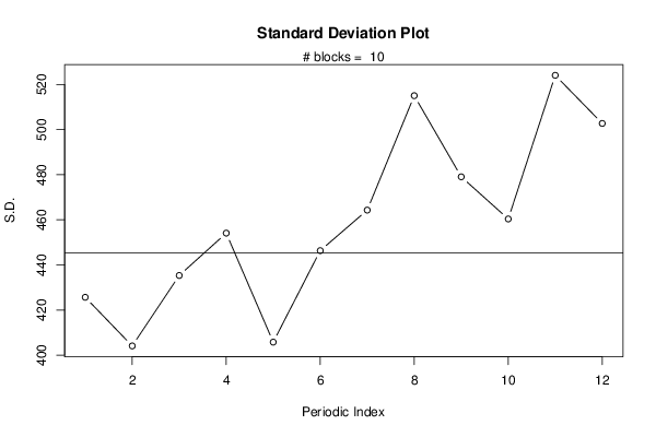
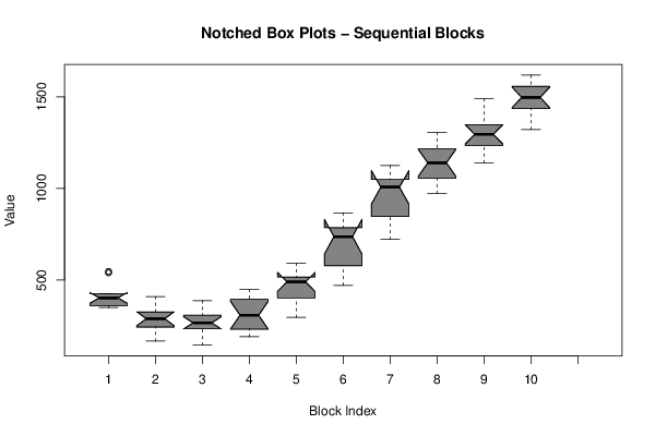
| Title produced by software | Standard Deviation Plot | ||||||||||||||||||||
| Date of computation | Fri, 12 Aug 2016 19:23:02 +0100 | ||||||||||||||||||||
| Cite this page as follows | Statistical Computations at FreeStatistics.org, Office for Research Development and Education, URL https://freestatistics.org/blog/index.php?v=date/2016/Aug/12/t1471026215ubv1ggjszk3syxf.htm/, Retrieved Sun, 05 May 2024 16:01:30 +0000 | ||||||||||||||||||||
| Statistical Computations at FreeStatistics.org, Office for Research Development and Education, URL https://freestatistics.org/blog/index.php?pk=296456, Retrieved Sun, 05 May 2024 16:01:30 +0000 | |||||||||||||||||||||
| QR Codes: | |||||||||||||||||||||
|
| |||||||||||||||||||||
| Original text written by user: | |||||||||||||||||||||
| IsPrivate? | No (this computation is public) | ||||||||||||||||||||
| User-defined keywords | |||||||||||||||||||||
| Estimated Impact | 115 | ||||||||||||||||||||
Tree of Dependent Computations | |||||||||||||||||||||
| Family? (F = Feedback message, R = changed R code, M = changed R Module, P = changed Parameters, D = changed Data) | |||||||||||||||||||||
| - [Univariate Data Series] [Omzet Mentos Aardbei] [2016-07-17 11:11:37] [74be16979710d4c4e7c6647856088456] - P [Univariate Data Series] [Omzet Mentos Aardbei] [2016-08-02 12:13:56] [74be16979710d4c4e7c6647856088456] - P [Univariate Data Series] [] [2016-08-12 10:07:18] [74be16979710d4c4e7c6647856088456] - R D [Univariate Data Series] [] [2016-08-12 10:23:50] [74be16979710d4c4e7c6647856088456] - RMP [Standard Deviation Plot] [] [2016-08-12 18:23:02] [d41d8cd98f00b204e9800998ecf8427e] [Current] | |||||||||||||||||||||
| Feedback Forum | |||||||||||||||||||||
Post a new message | |||||||||||||||||||||
Dataset | |||||||||||||||||||||
| Dataseries X: | |||||||||||||||||||||
425.25 417.75 410.25 395.25 546.75 539.25 425.25 349.50 357.00 357.00 364.50 380.25 334.50 288.75 251.25 251.25 395.25 410.25 296.25 167.25 235.50 235.50 288.75 319.50 312.00 235.50 273.75 258.75 387.75 357.00 235.50 144.75 228.00 251.25 273.75 303.75 243.00 190.50 213.00 220.50 417.75 417.75 303.75 288.75 334.50 312.00 372.75 448.50 463.50 357.00 327.00 296.25 501.75 516.75 478.50 516.75 509.25 448.50 516.75 592.50 623.25 531.75 471.00 516.75 714.00 774.75 759.75 789.75 782.25 706.50 835.50 866.25 911.25 774.75 721.50 782.25 927.00 1056.00 1025.25 1025.25 1040.25 987.75 1124.25 1124.25 1101.00 972.00 995.25 1010.25 1109.25 1238.25 1146.75 1192.50 1154.25 1131.75 1306.50 1268.25 1215.00 1139.25 1215.00 1253.25 1299.00 1359.75 1299.00 1336.50 1290.75 1283.25 1473.00 1488.75 1428.00 1321.50 1412.25 1450.50 1496.25 1564.50 1496.25 1549.50 1526.25 1443.00 1617.75 1617.75 | |||||||||||||||||||||
Tables (Output of Computation) | |||||||||||||||||||||
| |||||||||||||||||||||
Figures (Output of Computation) | |||||||||||||||||||||
Input Parameters & R Code | |||||||||||||||||||||
| Parameters (Session): | |||||||||||||||||||||
| par1 = 12 ; | |||||||||||||||||||||
| Parameters (R input): | |||||||||||||||||||||
| par1 = 12 ; | |||||||||||||||||||||
| R code (references can be found in the software module): | |||||||||||||||||||||
par1 <- as.numeric(par1) | |||||||||||||||||||||