Free Statistics
of Irreproducible Research!
Description of Statistical Computation | |||||||||||||||||||||
|---|---|---|---|---|---|---|---|---|---|---|---|---|---|---|---|---|---|---|---|---|---|
| Author's title | |||||||||||||||||||||
| Author | *Unverified author* | ||||||||||||||||||||
| R Software Module | rwasp_meanplot.wasp | ||||||||||||||||||||
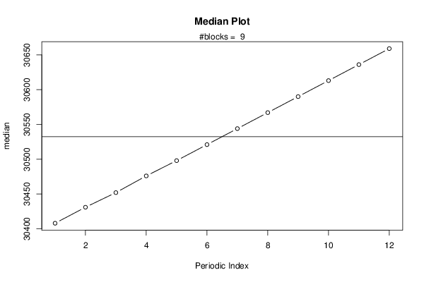
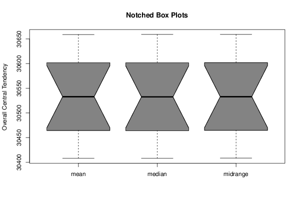
| Title produced by software | Mean Plot | ||||||||||||||||||||
| Date of computation | Sat, 13 Aug 2016 12:25:00 +0100 | ||||||||||||||||||||
| Cite this page as follows | Statistical Computations at FreeStatistics.org, Office for Research Development and Education, URL https://freestatistics.org/blog/index.php?v=date/2016/Aug/13/t1471087561swsedxgfdznm2rd.htm/, Retrieved Wed, 01 May 2024 20:21:45 +0000 | ||||||||||||||||||||
| Statistical Computations at FreeStatistics.org, Office for Research Development and Education, URL https://freestatistics.org/blog/index.php?pk=296505, Retrieved Wed, 01 May 2024 20:21:45 +0000 | |||||||||||||||||||||
| QR Codes: | |||||||||||||||||||||
|
| |||||||||||||||||||||
| Original text written by user: | |||||||||||||||||||||
| IsPrivate? | No (this computation is public) | ||||||||||||||||||||
| User-defined keywords | |||||||||||||||||||||
| Estimated Impact | 156 | ||||||||||||||||||||
Tree of Dependent Computations | |||||||||||||||||||||
| Family? (F = Feedback message, R = changed R code, M = changed R Module, P = changed Parameters, D = changed Data) | |||||||||||||||||||||
| - [Univariate Data Series] [] [2016-08-13 09:35:09] [74be16979710d4c4e7c6647856088456] - RMP [Mean Plot] [] [2016-08-13 11:25:00] [d41d8cd98f00b204e9800998ecf8427e] [Current] | |||||||||||||||||||||
| Feedback Forum | |||||||||||||||||||||
Post a new message | |||||||||||||||||||||
Dataset | |||||||||||||||||||||
| Dataseries X: | |||||||||||||||||||||
29312 29336 29357 29380 29402 29426 29448 29471 29495 29517 29540 29563 29586 29609 29631 29654 29677 29700 29723 29746 29769 29792 29815 29837 29861 29884 29905 29928 29951 29974 29996 30020 30043 30065 30089 30111 30134 30158 30179 30202 30224 30248 30270 30293 30317 30339 30362 30385 30408 30431 30452 30476 30498 30521 30544 30567 30590 30613 30636 30659 30682 30705 30727 30750 30773 30796 30818 30842 30865 30887 30911 30933 30956 30980 31001 31024 31046 31070 31092 31115 31139 31161 31184 31207 31230 31253 31274 31298 31320 31343 31366 31389 31412 31435 31458 31481 31504 31527 31548 31571 31594 31617 31640 31663 31686 31709 31732 31754 | |||||||||||||||||||||
Tables (Output of Computation) | |||||||||||||||||||||
| |||||||||||||||||||||
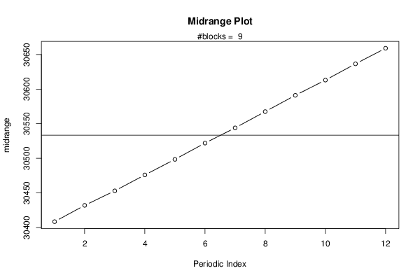
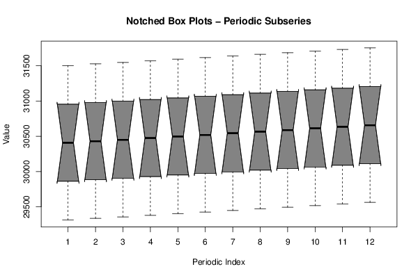
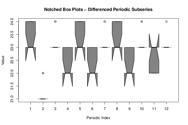
Figures (Output of Computation) | |||||||||||||||||||||
Input Parameters & R Code | |||||||||||||||||||||
| Parameters (Session): | |||||||||||||||||||||
| par1 = 12 ; | |||||||||||||||||||||
| Parameters (R input): | |||||||||||||||||||||
| par1 = 12 ; | |||||||||||||||||||||
| R code (references can be found in the software module): | |||||||||||||||||||||
par1 <- as.numeric(par1) | |||||||||||||||||||||