Repository of Reproducible Computations

Free Statistics

of Irreproducible Research!

Author's title

Author

*Unverified author*

R Software Module

rwasp_autocorrelation.wasp

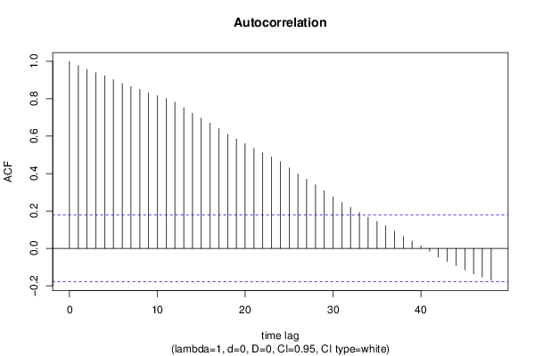
Title produced by software

(Partial) Autocorrelation Function

Date of computation

Mon, 15 Aug 2016 17:45:24 +0100

Cite this page as follows

Statistical Computations at FreeStatistics.org, Office for Research Development and Education, URL https://freestatistics.org/blog/index.php?v=date/2016/Aug/15/t1471279613psapvm7ewhzig9g.htm/, Retrieved Sat, 27 Apr 2024 19:43:34 +0200

Statistical Computations at FreeStatistics.org, Office for Research Development and Education, URL https://freestatistics.org/blog/index.php?pk=, Retrieved Sat, 27 Apr 2024 19:43:34 +0200

QR Codes:

Paste this QR Code to cite your computation.

Original text written by user:

IsPrivate?

No (this computation is public)

User-defined keywords

Estimated Impact

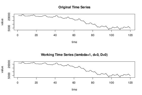
Dataseries X:

Download CSV

Histogram

Boxplots

Summary of computational transaction
Raw Input	view raw input (R code)
Raw Output	view raw output of R engine
Computing time	1 seconds
R Server	'Herman Ole Andreas Wold' @ wold.wessa.net
R Framework error message	Warning: there are blank lines in the 'Data' field. Please, use NA for missing data - blank lines are simply deleted and are NOT treated as missing values.

\begin{tabular}{lllllllll}
\hline
Summary of computational transaction \tabularnewline
Raw Input & view raw input (R code)  \tabularnewline
Raw Output & view raw output of R engine  \tabularnewline
Computing time & 1 seconds \tabularnewline
R Server & 'Herman Ole Andreas Wold' @ wold.wessa.net \tabularnewline
R Framework error message & Warning: there are blank lines in the 'Data' field.
Please, use NA for missing data - blank lines are simply
 deleted and are NOT treated as missing values. \tabularnewline
\hline
\end{tabular}
%Source: https://freestatistics.org/blog/index.php?pk=&T=0

[TABLE]
[ROW][C]Summary of computational transaction[/C][/ROW]
[ROW][C]Raw Input[/C][C]view raw input (R code) [/C][/ROW]
[ROW][C]Raw Output[/C][C]view raw output of R engine [/C][/ROW]
[ROW][C]Computing time[/C][C]1 seconds[/C][/ROW]
[ROW][C]R Server[/C][C]'Herman Ole Andreas Wold' @ wold.wessa.net[/C][/ROW]
[ROW][C]R Framework error message[/C][C]Warning: there are blank lines in the 'Data' field.
Please, use NA for missing data - blank lines are simply
 deleted and are NOT treated as missing values.[/C][/ROW]
[/TABLE]
Source: https://freestatistics.org/blog/index.php?pk=&T=0

Globally Unique Identifier (entire table): ba.freestatistics.org/blog/index.php?pk=&T=0

As an alternative you can also use a QR Code:

The GUIDs for individual cells are displayed in the table below:

Summary of computational transaction
Raw Input	view raw input (R code)
Raw Output	view raw output of R engine
Computing time	1 seconds
R Server	'Herman Ole Andreas Wold' @ wold.wessa.net
R Framework error message	Warning: there are blank lines in the 'Data' field. Please, use NA for missing data - blank lines are simply deleted and are NOT treated as missing values.

Autocorrelation Function
Time lag k	ACF(k)	T-STAT	P-value
1	0.977558	10.7086	0
2	0.956356	10.4764	0
3	0.938926	10.2854	0
4	0.922221	10.1024	0
5	0.902238	9.8835	0
6	0.881726	9.6588	0
7	0.864736	9.4727	0
8	0.849654	9.3075	0
9	0.831755	9.1114	0
10	0.81611	8.94	0
11	0.801825	8.7836	0
12	0.782382	8.5706	0
13	0.75241	8.2422	0
14	0.722632	7.916	0
15	0.696374	7.6284	0
16	0.669556	7.3346	0
17	0.640497	7.0163	0
18	0.61027	6.6852	0
19	0.584333	6.401	0
20	0.56048	6.1398	0
21	0.534341	5.8534	0
22	0.510138	5.5883	0
23	0.488866	5.3553	0
24	0.462512	5.0666	1e-06
25	0.429527	4.7052	3e-06
26	0.397718	4.3568	1.4e-05
27	0.369059	4.0428	4.7e-05
28	0.339647	3.7206	0.000152
29	0.307989	3.3739	0.000499
30	0.274758	3.0098	0.001593
31	0.245793	2.6925	0.004053
32	0.218906	2.398	0.009013
33	0.191995	2.1032	0.018769
34	0.166347	1.8222	0.035454
35	0.144367	1.5815	0.058203
36	0.120542	1.3205	0.094595
37	0.091943	1.0072	0.157936
38	0.06391	0.7001	0.242609
39	0.03891	0.4262	0.335349
40	0.013207	0.1447	0.442606
41	-0.015332	-0.168	0.43345
42	-0.045933	-0.5032	0.307883
43	-0.070215	-0.7692	0.221652
44	-0.092142	-1.0094	0.157415
45	-0.114844	-1.2581	0.105407
46	-0.135949	-1.4893	0.069522
47	-0.153201	-1.6782	0.047952
48	-0.170516	-1.8679	0.032107

\begin{tabular}{lllllllll}
\hline
Autocorrelation Function \tabularnewline
Time lag k & ACF(k) & T-STAT & P-value \tabularnewline
1 & 0.977558 & 10.7086 & 0 \tabularnewline
2 & 0.956356 & 10.4764 & 0 \tabularnewline
3 & 0.938926 & 10.2854 & 0 \tabularnewline
4 & 0.922221 & 10.1024 & 0 \tabularnewline
5 & 0.902238 & 9.8835 & 0 \tabularnewline
6 & 0.881726 & 9.6588 & 0 \tabularnewline
7 & 0.864736 & 9.4727 & 0 \tabularnewline
8 & 0.849654 & 9.3075 & 0 \tabularnewline
9 & 0.831755 & 9.1114 & 0 \tabularnewline
10 & 0.81611 & 8.94 & 0 \tabularnewline
11 & 0.801825 & 8.7836 & 0 \tabularnewline
12 & 0.782382 & 8.5706 & 0 \tabularnewline
13 & 0.75241 & 8.2422 & 0 \tabularnewline
14 & 0.722632 & 7.916 & 0 \tabularnewline
15 & 0.696374 & 7.6284 & 0 \tabularnewline
16 & 0.669556 & 7.3346 & 0 \tabularnewline
17 & 0.640497 & 7.0163 & 0 \tabularnewline
18 & 0.61027 & 6.6852 & 0 \tabularnewline
19 & 0.584333 & 6.401 & 0 \tabularnewline
20 & 0.56048 & 6.1398 & 0 \tabularnewline
21 & 0.534341 & 5.8534 & 0 \tabularnewline
22 & 0.510138 & 5.5883 & 0 \tabularnewline
23 & 0.488866 & 5.3553 & 0 \tabularnewline
24 & 0.462512 & 5.0666 & 1e-06 \tabularnewline
25 & 0.429527 & 4.7052 & 3e-06 \tabularnewline
26 & 0.397718 & 4.3568 & 1.4e-05 \tabularnewline
27 & 0.369059 & 4.0428 & 4.7e-05 \tabularnewline
28 & 0.339647 & 3.7206 & 0.000152 \tabularnewline
29 & 0.307989 & 3.3739 & 0.000499 \tabularnewline
30 & 0.274758 & 3.0098 & 0.001593 \tabularnewline
31 & 0.245793 & 2.6925 & 0.004053 \tabularnewline
32 & 0.218906 & 2.398 & 0.009013 \tabularnewline
33 & 0.191995 & 2.1032 & 0.018769 \tabularnewline
34 & 0.166347 & 1.8222 & 0.035454 \tabularnewline
35 & 0.144367 & 1.5815 & 0.058203 \tabularnewline
36 & 0.120542 & 1.3205 & 0.094595 \tabularnewline
37 & 0.091943 & 1.0072 & 0.157936 \tabularnewline
38 & 0.06391 & 0.7001 & 0.242609 \tabularnewline
39 & 0.03891 & 0.4262 & 0.335349 \tabularnewline
40 & 0.013207 & 0.1447 & 0.442606 \tabularnewline
41 & -0.015332 & -0.168 & 0.43345 \tabularnewline
42 & -0.045933 & -0.5032 & 0.307883 \tabularnewline
43 & -0.070215 & -0.7692 & 0.221652 \tabularnewline
44 & -0.092142 & -1.0094 & 0.157415 \tabularnewline
45 & -0.114844 & -1.2581 & 0.105407 \tabularnewline
46 & -0.135949 & -1.4893 & 0.069522 \tabularnewline
47 & -0.153201 & -1.6782 & 0.047952 \tabularnewline
48 & -0.170516 & -1.8679 & 0.032107 \tabularnewline
\hline
\end{tabular}
%Source: https://freestatistics.org/blog/index.php?pk=&T=1

[TABLE]
[ROW][C]Autocorrelation Function[/C][/ROW]
[ROW][C]Time lag k[/C][C]ACF(k)[/C][C]T-STAT[/C][C]P-value[/C][/ROW]
[ROW][C]1[/C][C]0.977558[/C][C]10.7086[/C][C]0[/C][/ROW]
[ROW][C]2[/C][C]0.956356[/C][C]10.4764[/C][C]0[/C][/ROW]
[ROW][C]3[/C][C]0.938926[/C][C]10.2854[/C][C]0[/C][/ROW]
[ROW][C]4[/C][C]0.922221[/C][C]10.1024[/C][C]0[/C][/ROW]
[ROW][C]5[/C][C]0.902238[/C][C]9.8835[/C][C]0[/C][/ROW]
[ROW][C]6[/C][C]0.881726[/C][C]9.6588[/C][C]0[/C][/ROW]
[ROW][C]7[/C][C]0.864736[/C][C]9.4727[/C][C]0[/C][/ROW]
[ROW][C]8[/C][C]0.849654[/C][C]9.3075[/C][C]0[/C][/ROW]
[ROW][C]9[/C][C]0.831755[/C][C]9.1114[/C][C]0[/C][/ROW]
[ROW][C]10[/C][C]0.81611[/C][C]8.94[/C][C]0[/C][/ROW]
[ROW][C]11[/C][C]0.801825[/C][C]8.7836[/C][C]0[/C][/ROW]
[ROW][C]12[/C][C]0.782382[/C][C]8.5706[/C][C]0[/C][/ROW]
[ROW][C]13[/C][C]0.75241[/C][C]8.2422[/C][C]0[/C][/ROW]
[ROW][C]14[/C][C]0.722632[/C][C]7.916[/C][C]0[/C][/ROW]
[ROW][C]15[/C][C]0.696374[/C][C]7.6284[/C][C]0[/C][/ROW]
[ROW][C]16[/C][C]0.669556[/C][C]7.3346[/C][C]0[/C][/ROW]
[ROW][C]17[/C][C]0.640497[/C][C]7.0163[/C][C]0[/C][/ROW]
[ROW][C]18[/C][C]0.61027[/C][C]6.6852[/C][C]0[/C][/ROW]
[ROW][C]19[/C][C]0.584333[/C][C]6.401[/C][C]0[/C][/ROW]
[ROW][C]20[/C][C]0.56048[/C][C]6.1398[/C][C]0[/C][/ROW]
[ROW][C]21[/C][C]0.534341[/C][C]5.8534[/C][C]0[/C][/ROW]
[ROW][C]22[/C][C]0.510138[/C][C]5.5883[/C][C]0[/C][/ROW]
[ROW][C]23[/C][C]0.488866[/C][C]5.3553[/C][C]0[/C][/ROW]
[ROW][C]24[/C][C]0.462512[/C][C]5.0666[/C][C]1e-06[/C][/ROW]
[ROW][C]25[/C][C]0.429527[/C][C]4.7052[/C][C]3e-06[/C][/ROW]
[ROW][C]26[/C][C]0.397718[/C][C]4.3568[/C][C]1.4e-05[/C][/ROW]
[ROW][C]27[/C][C]0.369059[/C][C]4.0428[/C][C]4.7e-05[/C][/ROW]
[ROW][C]28[/C][C]0.339647[/C][C]3.7206[/C][C]0.000152[/C][/ROW]
[ROW][C]29[/C][C]0.307989[/C][C]3.3739[/C][C]0.000499[/C][/ROW]
[ROW][C]30[/C][C]0.274758[/C][C]3.0098[/C][C]0.001593[/C][/ROW]
[ROW][C]31[/C][C]0.245793[/C][C]2.6925[/C][C]0.004053[/C][/ROW]
[ROW][C]32[/C][C]0.218906[/C][C]2.398[/C][C]0.009013[/C][/ROW]
[ROW][C]33[/C][C]0.191995[/C][C]2.1032[/C][C]0.018769[/C][/ROW]
[ROW][C]34[/C][C]0.166347[/C][C]1.8222[/C][C]0.035454[/C][/ROW]
[ROW][C]35[/C][C]0.144367[/C][C]1.5815[/C][C]0.058203[/C][/ROW]
[ROW][C]36[/C][C]0.120542[/C][C]1.3205[/C][C]0.094595[/C][/ROW]
[ROW][C]37[/C][C]0.091943[/C][C]1.0072[/C][C]0.157936[/C][/ROW]
[ROW][C]38[/C][C]0.06391[/C][C]0.7001[/C][C]0.242609[/C][/ROW]
[ROW][C]39[/C][C]0.03891[/C][C]0.4262[/C][C]0.335349[/C][/ROW]
[ROW][C]40[/C][C]0.013207[/C][C]0.1447[/C][C]0.442606[/C][/ROW]
[ROW][C]41[/C][C]-0.015332[/C][C]-0.168[/C][C]0.43345[/C][/ROW]
[ROW][C]42[/C][C]-0.045933[/C][C]-0.5032[/C][C]0.307883[/C][/ROW]
[ROW][C]43[/C][C]-0.070215[/C][C]-0.7692[/C][C]0.221652[/C][/ROW]
[ROW][C]44[/C][C]-0.092142[/C][C]-1.0094[/C][C]0.157415[/C][/ROW]
[ROW][C]45[/C][C]-0.114844[/C][C]-1.2581[/C][C]0.105407[/C][/ROW]
[ROW][C]46[/C][C]-0.135949[/C][C]-1.4893[/C][C]0.069522[/C][/ROW]
[ROW][C]47[/C][C]-0.153201[/C][C]-1.6782[/C][C]0.047952[/C][/ROW]
[ROW][C]48[/C][C]-0.170516[/C][C]-1.8679[/C][C]0.032107[/C][/ROW]
[/TABLE]
Source: https://freestatistics.org/blog/index.php?pk=&T=1

Globally Unique Identifier (entire table): ba.freestatistics.org/blog/index.php?pk=&T=1

As an alternative you can also use a QR Code:

The GUIDs for individual cells are displayed in the table below:

Autocorrelation Function
Time lag k	ACF(k)	T-STAT	P-value
1	0.977558	10.7086	0
2	0.956356	10.4764	0
3	0.938926	10.2854	0
4	0.922221	10.1024	0
5	0.902238	9.8835	0
6	0.881726	9.6588	0
7	0.864736	9.4727	0
8	0.849654	9.3075	0
9	0.831755	9.1114	0
10	0.81611	8.94	0
11	0.801825	8.7836	0
12	0.782382	8.5706	0
13	0.75241	8.2422	0
14	0.722632	7.916	0
15	0.696374	7.6284	0
16	0.669556	7.3346	0
17	0.640497	7.0163	0
18	0.61027	6.6852	0
19	0.584333	6.401	0
20	0.56048	6.1398	0
21	0.534341	5.8534	0
22	0.510138	5.5883	0
23	0.488866	5.3553	0
24	0.462512	5.0666	1e-06
25	0.429527	4.7052	3e-06
26	0.397718	4.3568	1.4e-05
27	0.369059	4.0428	4.7e-05
28	0.339647	3.7206	0.000152
29	0.307989	3.3739	0.000499
30	0.274758	3.0098	0.001593
31	0.245793	2.6925	0.004053
32	0.218906	2.398	0.009013
33	0.191995	2.1032	0.018769
34	0.166347	1.8222	0.035454
35	0.144367	1.5815	0.058203
36	0.120542	1.3205	0.094595
37	0.091943	1.0072	0.157936
38	0.06391	0.7001	0.242609
39	0.03891	0.4262	0.335349
40	0.013207	0.1447	0.442606
41	-0.015332	-0.168	0.43345
42	-0.045933	-0.5032	0.307883
43	-0.070215	-0.7692	0.221652
44	-0.092142	-1.0094	0.157415
45	-0.114844	-1.2581	0.105407
46	-0.135949	-1.4893	0.069522
47	-0.153201	-1.6782	0.047952
48	-0.170516	-1.8679	0.032107

Partial Autocorrelation Function
Time lag k	PACF(k)	T-STAT	P-value
1	0.977558	10.7086	0
2	0.016592	0.1818	0.428042
3	0.074923	0.8207	0.206712
4	0.01215	0.1331	0.447171
5	-0.074812	-0.8195	0.207056
6	-0.023522	-0.2577	0.398553
7	0.057624	0.6312	0.264541
8	0.034283	0.3756	0.353957
9	-0.054419	-0.5961	0.276106
10	0.049417	0.5413	0.294642
11	0.009415	0.1031	0.459012
12	-0.126698	-1.3879	0.083868
13	-0.246913	-2.7048	0.003914
14	-0.05006	-0.5484	0.292224
15	0.016773	0.1837	0.427264
16	-0.017788	-0.1949	0.422919
17	-0.020279	-0.2221	0.412288
18	-0.058051	-0.6359	0.26302
19	0.026763	0.2932	0.384946
20	0.020574	0.2254	0.411036
21	-0.041031	-0.4495	0.326951
22	0.015411	0.1688	0.433112
23	0.048924	0.5359	0.296498
24	-0.078675	-0.8618	0.195247
25	-0.116574	-1.277	0.102033
26	-0.017612	-0.1929	0.423672
27	-0.001899	-0.0208	0.49172
28	-0.0181	-0.1983	0.421582
29	-0.015032	-0.1647	0.434741
30	-0.07461	-0.8173	0.207686
31	-0.004405	-0.0483	0.480797
32	0.011736	0.1286	0.44896
33	0.009031	0.0989	0.46068
34	-0.013164	-0.1442	0.442791
35	0.057005	0.6245	0.266754
36	0.006234	0.0683	0.472834
37	-0.076341	-0.8363	0.202331
38	-0.030975	-0.3393	0.367482
39	-0.002742	-0.03	0.488042
40	-0.020652	-0.2262	0.410701
41	-0.024774	-0.2714	0.393279
42	-0.07178	-0.7863	0.216616
43	0.036621	0.4012	0.344506
44	0.011988	0.1313	0.447868
45	-0.014051	-0.1539	0.438965
46	-0.015053	-0.1649	0.43465
47	0.032013	0.3507	0.363222
48	0.018676	0.2046	0.419121

\begin{tabular}{lllllllll}
\hline
Partial Autocorrelation Function \tabularnewline
Time lag k & PACF(k) & T-STAT & P-value \tabularnewline
1 & 0.977558 & 10.7086 & 0 \tabularnewline
2 & 0.016592 & 0.1818 & 0.428042 \tabularnewline
3 & 0.074923 & 0.8207 & 0.206712 \tabularnewline
4 & 0.01215 & 0.1331 & 0.447171 \tabularnewline
5 & -0.074812 & -0.8195 & 0.207056 \tabularnewline
6 & -0.023522 & -0.2577 & 0.398553 \tabularnewline
7 & 0.057624 & 0.6312 & 0.264541 \tabularnewline
8 & 0.034283 & 0.3756 & 0.353957 \tabularnewline
9 & -0.054419 & -0.5961 & 0.276106 \tabularnewline
10 & 0.049417 & 0.5413 & 0.294642 \tabularnewline
11 & 0.009415 & 0.1031 & 0.459012 \tabularnewline
12 & -0.126698 & -1.3879 & 0.083868 \tabularnewline
13 & -0.246913 & -2.7048 & 0.003914 \tabularnewline
14 & -0.05006 & -0.5484 & 0.292224 \tabularnewline
15 & 0.016773 & 0.1837 & 0.427264 \tabularnewline
16 & -0.017788 & -0.1949 & 0.422919 \tabularnewline
17 & -0.020279 & -0.2221 & 0.412288 \tabularnewline
18 & -0.058051 & -0.6359 & 0.26302 \tabularnewline
19 & 0.026763 & 0.2932 & 0.384946 \tabularnewline
20 & 0.020574 & 0.2254 & 0.411036 \tabularnewline
21 & -0.041031 & -0.4495 & 0.326951 \tabularnewline
22 & 0.015411 & 0.1688 & 0.433112 \tabularnewline
23 & 0.048924 & 0.5359 & 0.296498 \tabularnewline
24 & -0.078675 & -0.8618 & 0.195247 \tabularnewline
25 & -0.116574 & -1.277 & 0.102033 \tabularnewline
26 & -0.017612 & -0.1929 & 0.423672 \tabularnewline
27 & -0.001899 & -0.0208 & 0.49172 \tabularnewline
28 & -0.0181 & -0.1983 & 0.421582 \tabularnewline
29 & -0.015032 & -0.1647 & 0.434741 \tabularnewline
30 & -0.07461 & -0.8173 & 0.207686 \tabularnewline
31 & -0.004405 & -0.0483 & 0.480797 \tabularnewline
32 & 0.011736 & 0.1286 & 0.44896 \tabularnewline
33 & 0.009031 & 0.0989 & 0.46068 \tabularnewline
34 & -0.013164 & -0.1442 & 0.442791 \tabularnewline
35 & 0.057005 & 0.6245 & 0.266754 \tabularnewline
36 & 0.006234 & 0.0683 & 0.472834 \tabularnewline
37 & -0.076341 & -0.8363 & 0.202331 \tabularnewline
38 & -0.030975 & -0.3393 & 0.367482 \tabularnewline
39 & -0.002742 & -0.03 & 0.488042 \tabularnewline
40 & -0.020652 & -0.2262 & 0.410701 \tabularnewline
41 & -0.024774 & -0.2714 & 0.393279 \tabularnewline
42 & -0.07178 & -0.7863 & 0.216616 \tabularnewline
43 & 0.036621 & 0.4012 & 0.344506 \tabularnewline
44 & 0.011988 & 0.1313 & 0.447868 \tabularnewline
45 & -0.014051 & -0.1539 & 0.438965 \tabularnewline
46 & -0.015053 & -0.1649 & 0.43465 \tabularnewline
47 & 0.032013 & 0.3507 & 0.363222 \tabularnewline
48 & 0.018676 & 0.2046 & 0.419121 \tabularnewline
\hline
\end{tabular}
%Source: https://freestatistics.org/blog/index.php?pk=&T=2

[TABLE]
[ROW][C]Partial Autocorrelation Function[/C][/ROW]
[ROW][C]Time lag k[/C][C]PACF(k)[/C][C]T-STAT[/C][C]P-value[/C][/ROW]
[ROW][C]1[/C][C]0.977558[/C][C]10.7086[/C][C]0[/C][/ROW]
[ROW][C]2[/C][C]0.016592[/C][C]0.1818[/C][C]0.428042[/C][/ROW]
[ROW][C]3[/C][C]0.074923[/C][C]0.8207[/C][C]0.206712[/C][/ROW]
[ROW][C]4[/C][C]0.01215[/C][C]0.1331[/C][C]0.447171[/C][/ROW]
[ROW][C]5[/C][C]-0.074812[/C][C]-0.8195[/C][C]0.207056[/C][/ROW]
[ROW][C]6[/C][C]-0.023522[/C][C]-0.2577[/C][C]0.398553[/C][/ROW]
[ROW][C]7[/C][C]0.057624[/C][C]0.6312[/C][C]0.264541[/C][/ROW]
[ROW][C]8[/C][C]0.034283[/C][C]0.3756[/C][C]0.353957[/C][/ROW]
[ROW][C]9[/C][C]-0.054419[/C][C]-0.5961[/C][C]0.276106[/C][/ROW]
[ROW][C]10[/C][C]0.049417[/C][C]0.5413[/C][C]0.294642[/C][/ROW]
[ROW][C]11[/C][C]0.009415[/C][C]0.1031[/C][C]0.459012[/C][/ROW]
[ROW][C]12[/C][C]-0.126698[/C][C]-1.3879[/C][C]0.083868[/C][/ROW]
[ROW][C]13[/C][C]-0.246913[/C][C]-2.7048[/C][C]0.003914[/C][/ROW]
[ROW][C]14[/C][C]-0.05006[/C][C]-0.5484[/C][C]0.292224[/C][/ROW]
[ROW][C]15[/C][C]0.016773[/C][C]0.1837[/C][C]0.427264[/C][/ROW]
[ROW][C]16[/C][C]-0.017788[/C][C]-0.1949[/C][C]0.422919[/C][/ROW]
[ROW][C]17[/C][C]-0.020279[/C][C]-0.2221[/C][C]0.412288[/C][/ROW]
[ROW][C]18[/C][C]-0.058051[/C][C]-0.6359[/C][C]0.26302[/C][/ROW]
[ROW][C]19[/C][C]0.026763[/C][C]0.2932[/C][C]0.384946[/C][/ROW]
[ROW][C]20[/C][C]0.020574[/C][C]0.2254[/C][C]0.411036[/C][/ROW]
[ROW][C]21[/C][C]-0.041031[/C][C]-0.4495[/C][C]0.326951[/C][/ROW]
[ROW][C]22[/C][C]0.015411[/C][C]0.1688[/C][C]0.433112[/C][/ROW]
[ROW][C]23[/C][C]0.048924[/C][C]0.5359[/C][C]0.296498[/C][/ROW]
[ROW][C]24[/C][C]-0.078675[/C][C]-0.8618[/C][C]0.195247[/C][/ROW]
[ROW][C]25[/C][C]-0.116574[/C][C]-1.277[/C][C]0.102033[/C][/ROW]
[ROW][C]26[/C][C]-0.017612[/C][C]-0.1929[/C][C]0.423672[/C][/ROW]
[ROW][C]27[/C][C]-0.001899[/C][C]-0.0208[/C][C]0.49172[/C][/ROW]
[ROW][C]28[/C][C]-0.0181[/C][C]-0.1983[/C][C]0.421582[/C][/ROW]
[ROW][C]29[/C][C]-0.015032[/C][C]-0.1647[/C][C]0.434741[/C][/ROW]
[ROW][C]30[/C][C]-0.07461[/C][C]-0.8173[/C][C]0.207686[/C][/ROW]
[ROW][C]31[/C][C]-0.004405[/C][C]-0.0483[/C][C]0.480797[/C][/ROW]
[ROW][C]32[/C][C]0.011736[/C][C]0.1286[/C][C]0.44896[/C][/ROW]
[ROW][C]33[/C][C]0.009031[/C][C]0.0989[/C][C]0.46068[/C][/ROW]
[ROW][C]34[/C][C]-0.013164[/C][C]-0.1442[/C][C]0.442791[/C][/ROW]
[ROW][C]35[/C][C]0.057005[/C][C]0.6245[/C][C]0.266754[/C][/ROW]
[ROW][C]36[/C][C]0.006234[/C][C]0.0683[/C][C]0.472834[/C][/ROW]
[ROW][C]37[/C][C]-0.076341[/C][C]-0.8363[/C][C]0.202331[/C][/ROW]
[ROW][C]38[/C][C]-0.030975[/C][C]-0.3393[/C][C]0.367482[/C][/ROW]
[ROW][C]39[/C][C]-0.002742[/C][C]-0.03[/C][C]0.488042[/C][/ROW]
[ROW][C]40[/C][C]-0.020652[/C][C]-0.2262[/C][C]0.410701[/C][/ROW]
[ROW][C]41[/C][C]-0.024774[/C][C]-0.2714[/C][C]0.393279[/C][/ROW]
[ROW][C]42[/C][C]-0.07178[/C][C]-0.7863[/C][C]0.216616[/C][/ROW]
[ROW][C]43[/C][C]0.036621[/C][C]0.4012[/C][C]0.344506[/C][/ROW]
[ROW][C]44[/C][C]0.011988[/C][C]0.1313[/C][C]0.447868[/C][/ROW]
[ROW][C]45[/C][C]-0.014051[/C][C]-0.1539[/C][C]0.438965[/C][/ROW]
[ROW][C]46[/C][C]-0.015053[/C][C]-0.1649[/C][C]0.43465[/C][/ROW]
[ROW][C]47[/C][C]0.032013[/C][C]0.3507[/C][C]0.363222[/C][/ROW]
[ROW][C]48[/C][C]0.018676[/C][C]0.2046[/C][C]0.419121[/C][/ROW]
[/TABLE]
Source: https://freestatistics.org/blog/index.php?pk=&T=2

Globally Unique Identifier (entire table): ba.freestatistics.org/blog/index.php?pk=&T=2

As an alternative you can also use a QR Code:

The GUIDs for individual cells are displayed in the table below:

Partial Autocorrelation Function
Time lag k	PACF(k)	T-STAT	P-value
1	0.977558	10.7086	0
2	0.016592	0.1818	0.428042
3	0.074923	0.8207	0.206712
4	0.01215	0.1331	0.447171
5	-0.074812	-0.8195	0.207056
6	-0.023522	-0.2577	0.398553
7	0.057624	0.6312	0.264541
8	0.034283	0.3756	0.353957
9	-0.054419	-0.5961	0.276106
10	0.049417	0.5413	0.294642
11	0.009415	0.1031	0.459012
12	-0.126698	-1.3879	0.083868
13	-0.246913	-2.7048	0.003914
14	-0.05006	-0.5484	0.292224
15	0.016773	0.1837	0.427264
16	-0.017788	-0.1949	0.422919
17	-0.020279	-0.2221	0.412288
18	-0.058051	-0.6359	0.26302
19	0.026763	0.2932	0.384946
20	0.020574	0.2254	0.411036
21	-0.041031	-0.4495	0.326951
22	0.015411	0.1688	0.433112
23	0.048924	0.5359	0.296498
24	-0.078675	-0.8618	0.195247
25	-0.116574	-1.277	0.102033
26	-0.017612	-0.1929	0.423672
27	-0.001899	-0.0208	0.49172
28	-0.0181	-0.1983	0.421582
29	-0.015032	-0.1647	0.434741
30	-0.07461	-0.8173	0.207686
31	-0.004405	-0.0483	0.480797
32	0.011736	0.1286	0.44896
33	0.009031	0.0989	0.46068
34	-0.013164	-0.1442	0.442791
35	0.057005	0.6245	0.266754
36	0.006234	0.0683	0.472834
37	-0.076341	-0.8363	0.202331
38	-0.030975	-0.3393	0.367482
39	-0.002742	-0.03	0.488042
40	-0.020652	-0.2262	0.410701
41	-0.024774	-0.2714	0.393279
42	-0.07178	-0.7863	0.216616
43	0.036621	0.4012	0.344506
44	0.011988	0.1313	0.447868
45	-0.014051	-0.1539	0.438965
46	-0.015053	-0.1649	0.43465
47	0.032013	0.3507	0.363222
48	0.018676	0.2046	0.419121

Figure 1

PNG link

Postscript link

PDF link

Figure 2

PNG link

Postscript link

PDF link

Figure 3

PNG link

Postscript link

PDF link

Parameters (Session):

par1 = 48 ; par2 = 1 ; par3 = 0 ; par4 = 0 ; par5 = 12 ; par6 = White Noise ; par7 = 0.95 ;

Parameters (R input):

par1 = 48 ; par2 = 1 ; par3 = 0 ; par4 = 0 ; par5 = 12 ; par6 = White Noise ; par7 = 0.95 ; par8 = ;

R code (references can be found in the software module):

if (par1 == 'Default') {
par1 = 10*log10(length(x))
} else {
par1 <- as.numeric(par1)
}
par2 <- as.numeric(par2)
par3 <- as.numeric(par3)
par4 <- as.numeric(par4)
par5 <- as.numeric(par5)
if (par6 == 'White Noise') par6 <- 'white' else par6 <- 'ma'
par7 <- as.numeric(par7)
if (par8 != '') par8 <- as.numeric(par8)
x <- na.omit(x)
ox <- x
if (par8 == '') {
if (par2 == 0) {
x <- log(x)
} else {
x <- (x ^ par2 - 1) / par2
}
} else {
x <- log(x,base=par8)
}
if (par3 > 0) x <- diff(x,lag=1,difference=par3)
if (par4 > 0) x <- diff(x,lag=par5,difference=par4)
bitmap(file='picts.png')
op <- par(mfrow=c(2,1))
plot(ox,type='l',main='Original Time Series',xlab='time',ylab='value')
if (par8=='') {
mytitle <- paste('Working Time Series (lambda=',par2,', d=',par3,', D=',par4,')',sep='')
mysub <- paste('(lambda=',par2,', d=',par3,', D=',par4,', CI=', par7, ', CI type=',par6,')',sep='')
} else {
mytitle <- paste('Working Time Series (base=',par8,', d=',par3,', D=',par4,')',sep='')
mysub <- paste('(base=',par8,', d=',par3,', D=',par4,', CI=', par7, ', CI type=',par6,')',sep='')
}
plot(x,type='l', main=mytitle,xlab='time',ylab='value')
par(op)
dev.off()
bitmap(file='pic1.png')
racf <- acf(x, par1, main='Autocorrelation', xlab='time lag', ylab='ACF', ci.type=par6, ci=par7, sub=mysub)
dev.off()
bitmap(file='pic2.png')
rpacf <- pacf(x,par1,main='Partial Autocorrelation',xlab='lags',ylab='PACF',sub=mysub)
dev.off()
(myacf <- c(racf$acf))
(mypacf <- c(rpacf$acf))
lengthx <- length(x)
sqrtn <- sqrt(lengthx)
load(file='createtable')
a<-table.start()
a<-table.row.start(a)
a<-table.element(a,'Autocorrelation Function',4,TRUE)
a<-table.row.end(a)
a<-table.row.start(a)
a<-table.element(a,'Time lag k',header=TRUE)
a<-table.element(a,hyperlink('basics.htm','ACF(k)','click here for more information about the Autocorrelation Function'),header=TRUE)
a<-table.element(a,'T-STAT',header=TRUE)
a<-table.element(a,'P-value',header=TRUE)
a<-table.row.end(a)
for (i in 2:(par1+1)) {
a<-table.row.start(a)
a<-table.element(a,i-1,header=TRUE)
a<-table.element(a,round(myacf[i],6))
mytstat <- myacf[i]*sqrtn
a<-table.element(a,round(mytstat,4))
a<-table.element(a,round(1-pt(abs(mytstat),lengthx),6))
a<-table.row.end(a)
}
a<-table.end(a)
table.save(a,file='mytable.tab')
a<-table.start()
a<-table.row.start(a)
a<-table.element(a,'Partial Autocorrelation Function',4,TRUE)
a<-table.row.end(a)
a<-table.row.start(a)
a<-table.element(a,'Time lag k',header=TRUE)
a<-table.element(a,hyperlink('basics.htm','PACF(k)','click here for more information about the Partial Autocorrelation Function'),header=TRUE)
a<-table.element(a,'T-STAT',header=TRUE)
a<-table.element(a,'P-value',header=TRUE)
a<-table.row.end(a)
for (i in 1:par1) {
a<-table.row.start(a)
a<-table.element(a,i,header=TRUE)
a<-table.element(a,round(mypacf[i],6))
mytstat <- mypacf[i]*sqrtn
a<-table.element(a,round(mytstat,4))
a<-table.element(a,round(1-pt(abs(mytstat),lengthx),6))
a<-table.row.end(a)
}
a<-table.end(a)
table.save(a,file='mytable1.tab')

Free Statistics

Description of Statistical Computation

Tree of Dependent Computations

Dataset

Tables (Output of Computation)

Figures (Output of Computation)

Input Parameters & R Code