Repository of Reproducible Computations

Free Statistics

of Irreproducible Research!

Author's title

Author

*The author of this computation has been verified*

R Software Module

rwasp_autocorrelation.wasp

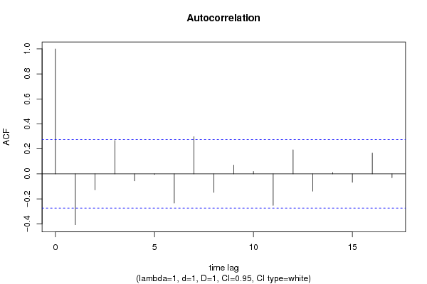
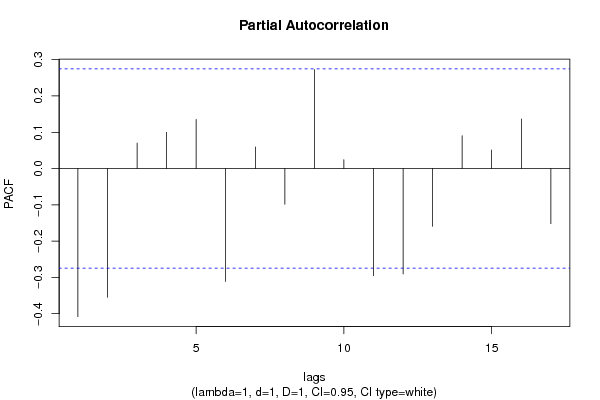
Title produced by software

(Partial) Autocorrelation Function

Date of computation

Wed, 07 Dec 2016 14:39:31 +0100

Cite this page as follows

Statistical Computations at FreeStatistics.org, Office for Research Development and Education, URL https://freestatistics.org/blog/index.php?v=date/2016/Dec/07/t148111802193xiwicxy277rwe.htm/, Retrieved Tue, 07 May 2024 20:00:14 +0000

Statistical Computations at FreeStatistics.org, Office for Research Development and Education, URL https://freestatistics.org/blog/index.php?pk=298104, Retrieved Tue, 07 May 2024 20:00:14 +0000

QR Codes:

Paste this QR Code to cite your computation.

Original text written by user:

IsPrivate?

No (this computation is public)

User-defined keywords

Estimated Impact

Family? (F = Feedback message, R = changed R code, M = changed R Module, P = changed Parameters, D = changed Data)

-       [(Partial) Autocorrelation Function] [Autocorr eerste] [2016-12-07 13:39:31] [4c05fa0998bf98e29c2e453b139976f4] [Current]
- RM      [Decomposition by Loess] [Loess 1e] [2016-12-09 13:34:56] [5f979cb1c6fa86b57093c7542788c28c] 
- RM      [Structural Time Series Models] [Structural Time S...] [2016-12-09 13:56:32] [5f979cb1c6fa86b57093c7542788c28c] 
- RM      [Exponential Smoothing] [smoothing eerste ] [2016-12-09 14:15:26] [5f979cb1c6fa86b57093c7542788c28c] 
- R  D    [(Partial) Autocorrelation Function] [kkeef] [2016-12-09 15:04:55] [5f979cb1c6fa86b57093c7542788c28c] 
- R  D    [(Partial) Autocorrelation Function] [skknfds] [2016-12-09 15:30:16] [5f979cb1c6fa86b57093c7542788c28c] 
- R  D    [(Partial) Autocorrelation Function] [lf,q] [2016-12-09 15:34:16] [5f979cb1c6fa86b57093c7542788c28c] 
- RM D    [Variance Reduction Matrix] [ksdn] [2016-12-09 15:38:37] [5f979cb1c6fa86b57093c7542788c28c] 
- RM D    [Structural Time Series Models] [qskndqld] [2016-12-09 15:42:30] [5f979cb1c6fa86b57093c7542788c28c] 
- RM D    [Exponential Smoothing] [Double] [2016-12-09 16:00:59] [5f979cb1c6fa86b57093c7542788c28c] 
- RM D    [Exponential Smoothing] [qlfns] [2016-12-09 16:04:27] [5f979cb1c6fa86b57093c7542788c28c] 

Feedback Forum

Post a new message

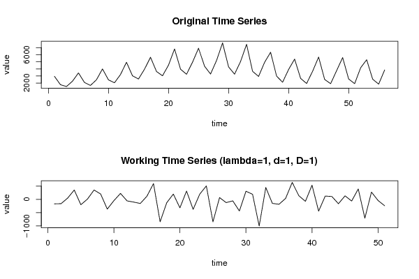
Dataseries X:

Download CSV

Histogram

Boxplots

Summary of computational transaction
Raw Input	view raw input (R code)
Raw Output	view raw output of R engine
Computing time	2 seconds
R Server	Big Analytics Cloud Computing Center

\begin{tabular}{lllllllll}
\hline
Summary of computational transaction \tabularnewline
Raw Input view raw input (R code)  \tabularnewline
Raw Outputview raw output of R engine  \tabularnewline
Computing time2 seconds \tabularnewline
R ServerBig Analytics Cloud Computing Center \tabularnewline
\hline
\end{tabular}
%Source: https://freestatistics.org/blog/index.php?pk=298104&T=0

[TABLE]
[ROW]

Summary of computational transaction[/C][/ROW] [ROW]

Raw Input[/C]

view raw input (R code) [/C][/ROW] [ROW]

Raw Output[/C]

view raw output of R engine [/C][/ROW] [ROW]

Computing time[/C]

2 seconds[/C][/ROW] [ROW]

R Server[/C]

Big Analytics Cloud Computing Center[/C][/ROW] [/TABLE] Source: https://freestatistics.org/blog/index.php?pk=298104&T=0

Globally Unique Identifier (entire table): ba.freestatistics.org/blog/index.php?pk=298104&T=0

As an alternative you can also use a QR Code:

The GUIDs for individual cells are displayed in the table below:

Summary of computational transaction
Raw Input	view raw input (R code)
Raw Output	view raw output of R engine
Computing time	2 seconds
R Server	Big Analytics Cloud Computing Center

Autocorrelation Function
Time lag k	ACF(k)	T-STAT	P-value
1	-0.40811	-2.9145	0.00264
2	-0.128938	-0.9208	0.180745
3	0.267	1.9068	0.031096
4	-0.056588	-0.4041	0.343907
5	-0.004924	-0.0352	0.486042
6	-0.233794	-1.6696	0.050561
7	0.297812	2.1268	0.019148
8	-0.148501	-1.0605	0.146956
9	0.070658	0.5046	0.308006
10	0.019576	0.1398	0.444684
11	-0.252424	-1.8027	0.038675
12	0.192226	1.3728	0.087916
13	-0.138319	-0.9878	0.163958
14	0.011118	0.0794	0.468512
15	-0.067389	-0.4813	0.316198
16	0.167302	1.1948	0.118851
17	-0.031197	-0.2228	0.412293

\begin{tabular}{lllllllll}
\hline
Autocorrelation Function \tabularnewline
Time lag k & ACF(k) & T-STAT & P-value \tabularnewline
1 & -0.40811 & -2.9145 & 0.00264 \tabularnewline
2 & -0.128938 & -0.9208 & 0.180745 \tabularnewline
3 & 0.267 & 1.9068 & 0.031096 \tabularnewline
4 & -0.056588 & -0.4041 & 0.343907 \tabularnewline
5 & -0.004924 & -0.0352 & 0.486042 \tabularnewline
6 & -0.233794 & -1.6696 & 0.050561 \tabularnewline
7 & 0.297812 & 2.1268 & 0.019148 \tabularnewline
8 & -0.148501 & -1.0605 & 0.146956 \tabularnewline
9 & 0.070658 & 0.5046 & 0.308006 \tabularnewline
10 & 0.019576 & 0.1398 & 0.444684 \tabularnewline
11 & -0.252424 & -1.8027 & 0.038675 \tabularnewline
12 & 0.192226 & 1.3728 & 0.087916 \tabularnewline
13 & -0.138319 & -0.9878 & 0.163958 \tabularnewline
14 & 0.011118 & 0.0794 & 0.468512 \tabularnewline
15 & -0.067389 & -0.4813 & 0.316198 \tabularnewline
16 & 0.167302 & 1.1948 & 0.118851 \tabularnewline
17 & -0.031197 & -0.2228 & 0.412293 \tabularnewline
\hline
\end{tabular}
%Source: https://freestatistics.org/blog/index.php?pk=298104&T=1

[TABLE]
[ROW][C]Autocorrelation Function[/C][/ROW]
[ROW][C]Time lag k[/C][C]ACF(k)[/C][C]T-STAT[/C][C]P-value[/C][/ROW]
[ROW][C]1[/C][C]-0.40811[/C][C]-2.9145[/C][C]0.00264[/C][/ROW]
[ROW][C]2[/C][C]-0.128938[/C][C]-0.9208[/C][C]0.180745[/C][/ROW]
[ROW][C]3[/C][C]0.267[/C][C]1.9068[/C][C]0.031096[/C][/ROW]
[ROW][C]4[/C][C]-0.056588[/C][C]-0.4041[/C][C]0.343907[/C][/ROW]
[ROW][C]5[/C][C]-0.004924[/C][C]-0.0352[/C][C]0.486042[/C][/ROW]
[ROW][C]6[/C][C]-0.233794[/C][C]-1.6696[/C][C]0.050561[/C][/ROW]
[ROW][C]7[/C][C]0.297812[/C][C]2.1268[/C][C]0.019148[/C][/ROW]
[ROW][C]8[/C][C]-0.148501[/C][C]-1.0605[/C][C]0.146956[/C][/ROW]
[ROW][C]9[/C][C]0.070658[/C][C]0.5046[/C][C]0.308006[/C][/ROW]
[ROW][C]10[/C][C]0.019576[/C][C]0.1398[/C][C]0.444684[/C][/ROW]
[ROW][C]11[/C][C]-0.252424[/C][C]-1.8027[/C][C]0.038675[/C][/ROW]
[ROW][C]12[/C][C]0.192226[/C][C]1.3728[/C][C]0.087916[/C][/ROW]
[ROW][C]13[/C][C]-0.138319[/C][C]-0.9878[/C][C]0.163958[/C][/ROW]
[ROW][C]14[/C][C]0.011118[/C][C]0.0794[/C][C]0.468512[/C][/ROW]
[ROW][C]15[/C][C]-0.067389[/C][C]-0.4813[/C][C]0.316198[/C][/ROW]
[ROW][C]16[/C][C]0.167302[/C][C]1.1948[/C][C]0.118851[/C][/ROW]
[ROW][C]17[/C][C]-0.031197[/C][C]-0.2228[/C][C]0.412293[/C][/ROW]
[/TABLE]
Source: https://freestatistics.org/blog/index.php?pk=298104&T=1

Globally Unique Identifier (entire table): ba.freestatistics.org/blog/index.php?pk=298104&T=1

As an alternative you can also use a QR Code:

The GUIDs for individual cells are displayed in the table below:

Autocorrelation Function
Time lag k	ACF(k)	T-STAT	P-value
1	-0.40811	-2.9145	0.00264
2	-0.128938	-0.9208	0.180745
3	0.267	1.9068	0.031096
4	-0.056588	-0.4041	0.343907
5	-0.004924	-0.0352	0.486042
6	-0.233794	-1.6696	0.050561
7	0.297812	2.1268	0.019148
8	-0.148501	-1.0605	0.146956
9	0.070658	0.5046	0.308006
10	0.019576	0.1398	0.444684
11	-0.252424	-1.8027	0.038675
12	0.192226	1.3728	0.087916
13	-0.138319	-0.9878	0.163958
14	0.011118	0.0794	0.468512
15	-0.067389	-0.4813	0.316198
16	0.167302	1.1948	0.118851
17	-0.031197	-0.2228	0.412293

Partial Autocorrelation Function
Time lag k	PACF(k)	T-STAT	P-value
1	-0.40811	-2.9145	0.00264
2	-0.354542	-2.5319	0.007233
3	0.070032	0.5001	0.309568
4	0.099626	0.7115	0.240016
5	0.135392	0.9669	0.169081
6	-0.310903	-2.2203	0.015435
7	0.059375	0.424	0.336665
8	-0.098284	-0.7019	0.242971
9	0.272715	1.9476	0.028491
10	0.024293	0.1735	0.431477
11	-0.295236	-2.1084	0.019964
12	-0.290371	-2.0737	0.02159
13	-0.159094	-1.1362	0.1306
14	0.090351	0.6452	0.260834
15	0.05111	0.365	0.358312
16	0.13643	0.9743	0.167252
17	-0.151844	-1.0844	0.141647

\begin{tabular}{lllllllll}
\hline
Partial Autocorrelation Function \tabularnewline
Time lag k & PACF(k) & T-STAT & P-value \tabularnewline
1 & -0.40811 & -2.9145 & 0.00264 \tabularnewline
2 & -0.354542 & -2.5319 & 0.007233 \tabularnewline
3 & 0.070032 & 0.5001 & 0.309568 \tabularnewline
4 & 0.099626 & 0.7115 & 0.240016 \tabularnewline
5 & 0.135392 & 0.9669 & 0.169081 \tabularnewline
6 & -0.310903 & -2.2203 & 0.015435 \tabularnewline
7 & 0.059375 & 0.424 & 0.336665 \tabularnewline
8 & -0.098284 & -0.7019 & 0.242971 \tabularnewline
9 & 0.272715 & 1.9476 & 0.028491 \tabularnewline
10 & 0.024293 & 0.1735 & 0.431477 \tabularnewline
11 & -0.295236 & -2.1084 & 0.019964 \tabularnewline
12 & -0.290371 & -2.0737 & 0.02159 \tabularnewline
13 & -0.159094 & -1.1362 & 0.1306 \tabularnewline
14 & 0.090351 & 0.6452 & 0.260834 \tabularnewline
15 & 0.05111 & 0.365 & 0.358312 \tabularnewline
16 & 0.13643 & 0.9743 & 0.167252 \tabularnewline
17 & -0.151844 & -1.0844 & 0.141647 \tabularnewline
\hline
\end{tabular}
%Source: https://freestatistics.org/blog/index.php?pk=298104&T=2

[TABLE]
[ROW][C]Partial Autocorrelation Function[/C][/ROW]
[ROW][C]Time lag k[/C][C]PACF(k)[/C][C]T-STAT[/C][C]P-value[/C][/ROW]
[ROW][C]1[/C][C]-0.40811[/C][C]-2.9145[/C][C]0.00264[/C][/ROW]
[ROW][C]2[/C][C]-0.354542[/C][C]-2.5319[/C][C]0.007233[/C][/ROW]
[ROW][C]3[/C][C]0.070032[/C][C]0.5001[/C][C]0.309568[/C][/ROW]
[ROW][C]4[/C][C]0.099626[/C][C]0.7115[/C][C]0.240016[/C][/ROW]
[ROW][C]5[/C][C]0.135392[/C][C]0.9669[/C][C]0.169081[/C][/ROW]
[ROW][C]6[/C][C]-0.310903[/C][C]-2.2203[/C][C]0.015435[/C][/ROW]
[ROW][C]7[/C][C]0.059375[/C][C]0.424[/C][C]0.336665[/C][/ROW]
[ROW][C]8[/C][C]-0.098284[/C][C]-0.7019[/C][C]0.242971[/C][/ROW]
[ROW][C]9[/C][C]0.272715[/C][C]1.9476[/C][C]0.028491[/C][/ROW]
[ROW][C]10[/C][C]0.024293[/C][C]0.1735[/C][C]0.431477[/C][/ROW]
[ROW][C]11[/C][C]-0.295236[/C][C]-2.1084[/C][C]0.019964[/C][/ROW]
[ROW][C]12[/C][C]-0.290371[/C][C]-2.0737[/C][C]0.02159[/C][/ROW]
[ROW][C]13[/C][C]-0.159094[/C][C]-1.1362[/C][C]0.1306[/C][/ROW]
[ROW][C]14[/C][C]0.090351[/C][C]0.6452[/C][C]0.260834[/C][/ROW]
[ROW][C]15[/C][C]0.05111[/C][C]0.365[/C][C]0.358312[/C][/ROW]
[ROW][C]16[/C][C]0.13643[/C][C]0.9743[/C][C]0.167252[/C][/ROW]
[ROW][C]17[/C][C]-0.151844[/C][C]-1.0844[/C][C]0.141647[/C][/ROW]
[/TABLE]
Source: https://freestatistics.org/blog/index.php?pk=298104&T=2

Globally Unique Identifier (entire table): ba.freestatistics.org/blog/index.php?pk=298104&T=2

As an alternative you can also use a QR Code:

The GUIDs for individual cells are displayed in the table below:

Partial Autocorrelation Function
Time lag k	PACF(k)	T-STAT	P-value
1	-0.40811	-2.9145	0.00264
2	-0.354542	-2.5319	0.007233
3	0.070032	0.5001	0.309568
4	0.099626	0.7115	0.240016
5	0.135392	0.9669	0.169081
6	-0.310903	-2.2203	0.015435
7	0.059375	0.424	0.336665
8	-0.098284	-0.7019	0.242971
9	0.272715	1.9476	0.028491
10	0.024293	0.1735	0.431477
11	-0.295236	-2.1084	0.019964
12	-0.290371	-2.0737	0.02159
13	-0.159094	-1.1362	0.1306
14	0.090351	0.6452	0.260834
15	0.05111	0.365	0.358312
16	0.13643	0.9743	0.167252
17	-0.151844	-1.0844	0.141647

Figure 1

PNG link

Postscript link

PDF link

Figure 2

PNG link

Postscript link

PDF link

Figure 3

PNG link

Postscript link

PDF link

Parameters (Session):

par1 = Default ; par2 = 1 ; par3 = 1 ; par4 = 1 ; par5 = 4 ; par6 = White Noise ; par7 = 0.95 ;

Parameters (R input):

par1 = Default ; par2 = 1 ; par3 = 1 ; par4 = 1 ; par5 = 4 ; par6 = White Noise ; par7 = 0.95 ; par8 = ;

R code (references can be found in the software module):

par8 <- ''
par7 <- '0.95'
par6 <- 'White Noise'
par5 <- '4'
par4 <- '1'
par3 <- '1'
par2 <- '1'
par1 <- 'Default'
if (par1 == 'Default') {
par1 = 10*log10(length(x))
} else {
par1 <- as.numeric(par1)
}
par2 <- as.numeric(par2)
par3 <- as.numeric(par3)
par4 <- as.numeric(par4)
par5 <- as.numeric(par5)
if (par6 == 'White Noise') par6 <- 'white' else par6 <- 'ma'
par7 <- as.numeric(par7)
if (par8 != '') par8 <- as.numeric(par8)
x <- na.omit(x)
ox <- x
if (par8 == '') {
if (par2 == 0) {
x <- log(x)
} else {
x <- (x ^ par2 - 1) / par2
}
} else {
x <- log(x,base=par8)
}
if (par3 > 0) x <- diff(x,lag=1,difference=par3)
if (par4 > 0) x <- diff(x,lag=par5,difference=par4)
bitmap(file='picts.png')
op <- par(mfrow=c(2,1))
plot(ox,type='l',main='Original Time Series',xlab='time',ylab='value')
if (par8=='') {
mytitle <- paste('Working Time Series (lambda=',par2,', d=',par3,', D=',par4,')',sep='')
mysub <- paste('(lambda=',par2,', d=',par3,', D=',par4,', CI=', par7, ', CI type=',par6,')',sep='')
} else {
mytitle <- paste('Working Time Series (base=',par8,', d=',par3,', D=',par4,')',sep='')
mysub <- paste('(base=',par8,', d=',par3,', D=',par4,', CI=', par7, ', CI type=',par6,')',sep='')
}
plot(x,type='l', main=mytitle,xlab='time',ylab='value')
par(op)
dev.off()
bitmap(file='pic1.png')
racf <- acf(x, par1, main='Autocorrelation', xlab='time lag', ylab='ACF', ci.type=par6, ci=par7, sub=mysub)
dev.off()
bitmap(file='pic2.png')
rpacf <- pacf(x,par1,main='Partial Autocorrelation',xlab='lags',ylab='PACF',sub=mysub)
dev.off()
(myacf <- c(racf$acf))
(mypacf <- c(rpacf$acf))
lengthx <- length(x)
sqrtn <- sqrt(lengthx)
load(file='createtable')
a<-table.start()
a<-table.row.start(a)
a<-table.element(a,'Autocorrelation Function',4,TRUE)
a<-table.row.end(a)
a<-table.row.start(a)
a<-table.element(a,'Time lag k',header=TRUE)
a<-table.element(a,'ACF(k)',header=TRUE)
a<-table.element(a,'T-STAT',header=TRUE)
a<-table.element(a,'P-value',header=TRUE)
a<-table.row.end(a)
for (i in 2:(par1+1)) {
a<-table.row.start(a)
a<-table.element(a,i-1,header=TRUE)
a<-table.element(a,round(myacf[i],6))
mytstat <- myacf[i]*sqrtn
a<-table.element(a,round(mytstat,4))
a<-table.element(a,round(1-pt(abs(mytstat),lengthx),6))
a<-table.row.end(a)
}
a<-table.end(a)
table.save(a,file='mytable.tab')
a<-table.start()
a<-table.row.start(a)
a<-table.element(a,'Partial Autocorrelation Function',4,TRUE)
a<-table.row.end(a)
a<-table.row.start(a)
a<-table.element(a,'Time lag k',header=TRUE)
a<-table.element(a,'PACF(k)',header=TRUE)
a<-table.element(a,'T-STAT',header=TRUE)
a<-table.element(a,'P-value',header=TRUE)
a<-table.row.end(a)
for (i in 1:par1) {
a<-table.row.start(a)
a<-table.element(a,i,header=TRUE)
a<-table.element(a,round(mypacf[i],6))
mytstat <- mypacf[i]*sqrtn
a<-table.element(a,round(mytstat,4))
a<-table.element(a,round(1-pt(abs(mytstat),lengthx),6))
a<-table.row.end(a)
}
a<-table.end(a)
table.save(a,file='mytable1.tab')

Free Statistics

Description of Statistical Computation

Tree of Dependent Computations

Dataset

Tables (Output of Computation)

Figures (Output of Computation)

Input Parameters & R Code