Repository of Reproducible Computations

Free Statistics

of Irreproducible Research!

Author's title

Author

*The author of this computation has been verified*

R Software Module

rwasp_arimaforecasting.wasp

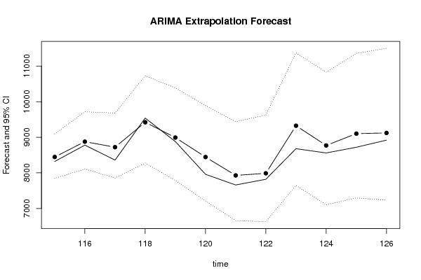
Title produced by software

ARIMA Forecasting

Date of computation

Thu, 15 Dec 2016 20:00:32 +0100

Cite this page as follows

Statistical Computations at FreeStatistics.org, Office for Research Development and Education, URL https://freestatistics.org/blog/index.php?v=date/2016/Dec/15/t14818295901wziahqb19wuicq.htm/, Retrieved Fri, 03 May 2024 06:26:50 +0000

Statistical Computations at FreeStatistics.org, Office for Research Development and Education, URL https://freestatistics.org/blog/index.php?pk=299970, Retrieved Fri, 03 May 2024 06:26:50 +0000

QR Codes:

Paste this QR Code to cite your computation.

Original text written by user:

IsPrivate?

No (this computation is public)

User-defined keywords

Estimated Impact

Family? (F = Feedback message, R = changed R code, M = changed R Module, P = changed Parameters, D = changed Data)

-       [ARIMA Forecasting] [ ARIMA FORECAST] [2016-12-15 19:00:32] [b95f76f605693b3a3343a287ab24f42a] [Current]
- RMP     [(Partial) Autocorrelation Function] [AUtocorrelation ] [2016-12-18 19:08:03] [d1d385d9b7e195437bdc484ddbefdda4] 
- RMPD    [ARIMA Backward Selection] [Arima Backward Se...] [2016-12-19 20:48:05] [d1d385d9b7e195437bdc484ddbefdda4] 
- RMP       [ARIMA Forecasting] [Arima Forecast new ] [2016-12-21 12:59:28] [d1d385d9b7e195437bdc484ddbefdda4] 
- R           [ARIMA Forecasting] [Arima forecast ge...] [2016-12-22 20:17:05] [d1d385d9b7e195437bdc484ddbefdda4] 
- RM          [Variance Reduction Matrix] [Variance Reductio...] [2016-12-23 08:50:27] [d1d385d9b7e195437bdc484ddbefdda4] 
- RMP       [Standard Deviation-Mean Plot] [Standard Deviation ] [2016-12-21 13:08:00] [d1d385d9b7e195437bdc484ddbefdda4] 
-   P       [ARIMA Backward Selection] [Backward Selection ] [2016-12-21 13:12:29] [d1d385d9b7e195437bdc484ddbefdda4] 
-             [ARIMA Backward Selection] [BAckward last] [2016-12-23 09:25:09] [d1d385d9b7e195437bdc484ddbefdda4] 
- R PD    [ARIMA Forecasting] [Arima Forecast me...] [2016-12-19 22:10:16] [d1d385d9b7e195437bdc484ddbefdda4] 
- RMPD    [One Sample Tests about the Mean] [Vraag 1] [2016-12-21 09:55:07] [d1d385d9b7e195437bdc484ddbefdda4] 
- RMPD    [Skewness and Kurtosis Test] [Vraag 2] [2016-12-21 10:00:47] [d1d385d9b7e195437bdc484ddbefdda4] 
- RMPD    [Central Tendency] [Vraag 3] [2016-12-21 10:09:51] [d1d385d9b7e195437bdc484ddbefdda4] 
- RMPD    [Two-Way ANOVA] [VRaag 4] [2016-12-21 10:23:53] [d1d385d9b7e195437bdc484ddbefdda4] 
- RMPD    [Chi-Squared Test, McNemar Test, and Fisher Exact Test] [Vraag 5] [2016-12-21 10:30:34] [d1d385d9b7e195437bdc484ddbefdda4] 
- RMPD    [Standard Deviation-Mean Plot] [VRaag 6.1] [2016-12-21 10:37:42] [d1d385d9b7e195437bdc484ddbefdda4] 
- RMPD    [Variance Reduction Matrix] [VRaag 6.2] [2016-12-21 10:40:18] [d1d385d9b7e195437bdc484ddbefdda4] 
- RMPD    [ARIMA Backward Selection] [VRaag 6.3] [2016-12-21 10:47:44] [d1d385d9b7e195437bdc484ddbefdda4] 
- R PD    [ARIMA Forecasting] [VRaag 7] [2016-12-21 10:55:44] [d1d385d9b7e195437bdc484ddbefdda4] 

Feedback Forum

Post a new message

Dataseries X:

Download CSV

Histogram

Boxplots

Summary of computational transaction
Raw Input	view raw input (R code)
Raw Output	view raw output of R engine
Computing time	1 seconds
R Server	Big Analytics Cloud Computing Center

\begin{tabular}{lllllllll}
\hline
Summary of computational transaction \tabularnewline
Raw Input view raw input (R code)  \tabularnewline
Raw Outputview raw output of R engine  \tabularnewline
Computing time1 seconds \tabularnewline
R ServerBig Analytics Cloud Computing Center \tabularnewline
\hline
\end{tabular}
%Source: https://freestatistics.org/blog/index.php?pk=299970&T=0

[TABLE]
[ROW]

Summary of computational transaction[/C][/ROW] [ROW]

Raw Input[/C]

view raw input (R code) [/C][/ROW] [ROW]

Raw Output[/C]

view raw output of R engine [/C][/ROW] [ROW]

Computing time[/C]

1 seconds[/C][/ROW] [ROW]

R Server[/C]

Big Analytics Cloud Computing Center[/C][/ROW] [/TABLE] Source: https://freestatistics.org/blog/index.php?pk=299970&T=0

Globally Unique Identifier (entire table): ba.freestatistics.org/blog/index.php?pk=299970&T=0

As an alternative you can also use a QR Code:

The GUIDs for individual cells are displayed in the table below:

Summary of computational transaction
Raw Input	view raw input (R code)
Raw Output	view raw output of R engine
Computing time	1 seconds
R Server	Big Analytics Cloud Computing Center

Univariate ARIMA Extrapolation Forecast
time	Y[t]	F[t]	95% LB	95% UB	p-value(H0: Y[t] = F[t])	P(F[t]>Y[t-1])	P(F[t]>Y[t-s])	P(F[t]>Y[114])
102	8640	-	-	-	-	-	-	-
103	8340	-	-	-	-	-	-	-
104	9100	-	-	-	-	-	-	-
105	8719.99999999999	-	-	-	-	-	-	-
106	9360	-	-	-	-	-	-	-
107	8800.00000000001	-	-	-	-	-	-	-
108	8060	-	-	-	-	-	-	-
109	7379.99999999999	-	-	-	-	-	-	-
110	7040	-	-	-	-	-	-	-
111	8020	-	-	-	-	-	-	-
112	7800	-	-	-	-	-	-	-
113	8380	-	-	-	-	-	-	-
114	8480	-	-	-	-	-	-	-
115	8320	8446.3662	7846.0836	9092.5748	0.3508	0.4594	0.6265	0.4594
116	8780	8876.9982	8109.5279	9717.1004	0.4105	0.9031	0.3014	0.8228
117	8360	8721.6866	7856.2314	9682.4816	0.2303	0.4527	0.5014	0.689
118	9540	9422.6715	8276.2599	10727.8818	0.4301	0.9447	0.5375	0.9216
119	8880	8992.6357	7784.3116	10388.5225	0.4372	0.2211	0.6066	0.7642
120	7960	8444.7421	7208.3513	9893.2013	0.2559	0.2779	0.6987	0.481
121	7660	7928.7723	6659.7148	9439.658	0.3637	0.4838	0.7617	0.2373
122	7820	7988.6251	6629.0467	9627.0451	0.4201	0.6529	0.8718	0.2783
123	8680	9325.2138	7645.7271	11373.6223	0.2685	0.9251	0.8941	0.7907
124	8560	8770.8191	7104.2278	10828.3785	0.4204	0.5345	0.8225	0.6091
125	8720	9102.9264	7295.6491	11357.9023	0.3696	0.6815	0.7351	0.7059
126	8920	9122.667	7235.4852	11502.0695	0.4337	0.6299	0.7017	0.7017

\begin{tabular}{lllllllll}
\hline
Univariate ARIMA Extrapolation Forecast \tabularnewline
time & Y[t] & F[t] & 95% LB & 95% UB & p-value(H0: Y[t] = F[t]) & P(F[t]>Y[t-1]) & P(F[t]>Y[t-s]) & P(F[t]>Y[114]) \tabularnewline
102 & 8640 & - & - & - & - & - & - & - \tabularnewline
103 & 8340 & - & - & - & - & - & - & - \tabularnewline
104 & 9100 & - & - & - & - & - & - & - \tabularnewline
105 & 8719.99999999999 & - & - & - & - & - & - & - \tabularnewline
106 & 9360 & - & - & - & - & - & - & - \tabularnewline
107 & 8800.00000000001 & - & - & - & - & - & - & - \tabularnewline
108 & 8060 & - & - & - & - & - & - & - \tabularnewline
109 & 7379.99999999999 & - & - & - & - & - & - & - \tabularnewline
110 & 7040 & - & - & - & - & - & - & - \tabularnewline
111 & 8020 & - & - & - & - & - & - & - \tabularnewline
112 & 7800 & - & - & - & - & - & - & - \tabularnewline
113 & 8380 & - & - & - & - & - & - & - \tabularnewline
114 & 8480 & - & - & - & - & - & - & - \tabularnewline
115 & 8320 & 8446.3662 & 7846.0836 & 9092.5748 & 0.3508 & 0.4594 & 0.6265 & 0.4594 \tabularnewline
116 & 8780 & 8876.9982 & 8109.5279 & 9717.1004 & 0.4105 & 0.9031 & 0.3014 & 0.8228 \tabularnewline
117 & 8360 & 8721.6866 & 7856.2314 & 9682.4816 & 0.2303 & 0.4527 & 0.5014 & 0.689 \tabularnewline
118 & 9540 & 9422.6715 & 8276.2599 & 10727.8818 & 0.4301 & 0.9447 & 0.5375 & 0.9216 \tabularnewline
119 & 8880 & 8992.6357 & 7784.3116 & 10388.5225 & 0.4372 & 0.2211 & 0.6066 & 0.7642 \tabularnewline
120 & 7960 & 8444.7421 & 7208.3513 & 9893.2013 & 0.2559 & 0.2779 & 0.6987 & 0.481 \tabularnewline
121 & 7660 & 7928.7723 & 6659.7148 & 9439.658 & 0.3637 & 0.4838 & 0.7617 & 0.2373 \tabularnewline
122 & 7820 & 7988.6251 & 6629.0467 & 9627.0451 & 0.4201 & 0.6529 & 0.8718 & 0.2783 \tabularnewline
123 & 8680 & 9325.2138 & 7645.7271 & 11373.6223 & 0.2685 & 0.9251 & 0.8941 & 0.7907 \tabularnewline
124 & 8560 & 8770.8191 & 7104.2278 & 10828.3785 & 0.4204 & 0.5345 & 0.8225 & 0.6091 \tabularnewline
125 & 8720 & 9102.9264 & 7295.6491 & 11357.9023 & 0.3696 & 0.6815 & 0.7351 & 0.7059 \tabularnewline
126 & 8920 & 9122.667 & 7235.4852 & 11502.0695 & 0.4337 & 0.6299 & 0.7017 & 0.7017 \tabularnewline
\hline
\end{tabular}
%Source: https://freestatistics.org/blog/index.php?pk=299970&T=1

[TABLE]
[ROW][C]Univariate ARIMA Extrapolation Forecast[/C][/ROW]
[ROW][C]time[/C][C]Y[t][/C][C]F[t][/C][C]95% LB[/C][C]95% UB[/C][C]p-value(H0: Y[t] = F[t])[/C][C]P(F[t]>Y[t-1])[/C][C]P(F[t]>Y[t-s])[/C][C]P(F[t]>Y[114])[/C][/ROW]
[ROW][C]102[/C][C]8640[/C][C]-[/C][C]-[/C][C]-[/C][C]-[/C][C]-[/C][C]-[/C][C]-[/C][/ROW]
[ROW][C]103[/C][C]8340[/C][C]-[/C][C]-[/C][C]-[/C][C]-[/C][C]-[/C][C]-[/C][C]-[/C][/ROW]
[ROW][C]104[/C][C]9100[/C][C]-[/C][C]-[/C][C]-[/C][C]-[/C][C]-[/C][C]-[/C][C]-[/C][/ROW]
[ROW][C]105[/C][C]8719.99999999999[/C][C]-[/C][C]-[/C][C]-[/C][C]-[/C][C]-[/C][C]-[/C][C]-[/C][/ROW]
[ROW][C]106[/C][C]9360[/C][C]-[/C][C]-[/C][C]-[/C][C]-[/C][C]-[/C][C]-[/C][C]-[/C][/ROW]
[ROW][C]107[/C][C]8800.00000000001[/C][C]-[/C][C]-[/C][C]-[/C][C]-[/C][C]-[/C][C]-[/C][C]-[/C][/ROW]
[ROW][C]108[/C][C]8060[/C][C]-[/C][C]-[/C][C]-[/C][C]-[/C][C]-[/C][C]-[/C][C]-[/C][/ROW]
[ROW][C]109[/C][C]7379.99999999999[/C][C]-[/C][C]-[/C][C]-[/C][C]-[/C][C]-[/C][C]-[/C][C]-[/C][/ROW]
[ROW][C]110[/C][C]7040[/C][C]-[/C][C]-[/C][C]-[/C][C]-[/C][C]-[/C][C]-[/C][C]-[/C][/ROW]
[ROW][C]111[/C][C]8020[/C][C]-[/C][C]-[/C][C]-[/C][C]-[/C][C]-[/C][C]-[/C][C]-[/C][/ROW]
[ROW][C]112[/C][C]7800[/C][C]-[/C][C]-[/C][C]-[/C][C]-[/C][C]-[/C][C]-[/C][C]-[/C][/ROW]
[ROW][C]113[/C][C]8380[/C][C]-[/C][C]-[/C][C]-[/C][C]-[/C][C]-[/C][C]-[/C][C]-[/C][/ROW]
[ROW][C]114[/C][C]8480[/C][C]-[/C][C]-[/C][C]-[/C][C]-[/C][C]-[/C][C]-[/C][C]-[/C][/ROW]
[ROW][C]115[/C][C]8320[/C][C]8446.3662[/C][C]7846.0836[/C][C]9092.5748[/C][C]0.3508[/C][C]0.4594[/C][C]0.6265[/C][C]0.4594[/C][/ROW]
[ROW][C]116[/C][C]8780[/C][C]8876.9982[/C][C]8109.5279[/C][C]9717.1004[/C][C]0.4105[/C][C]0.9031[/C][C]0.3014[/C][C]0.8228[/C][/ROW]
[ROW][C]117[/C][C]8360[/C][C]8721.6866[/C][C]7856.2314[/C][C]9682.4816[/C][C]0.2303[/C][C]0.4527[/C][C]0.5014[/C][C]0.689[/C][/ROW]
[ROW][C]118[/C][C]9540[/C][C]9422.6715[/C][C]8276.2599[/C][C]10727.8818[/C][C]0.4301[/C][C]0.9447[/C][C]0.5375[/C][C]0.9216[/C][/ROW]
[ROW][C]119[/C][C]8880[/C][C]8992.6357[/C][C]7784.3116[/C][C]10388.5225[/C][C]0.4372[/C][C]0.2211[/C][C]0.6066[/C][C]0.7642[/C][/ROW]
[ROW][C]120[/C][C]7960[/C][C]8444.7421[/C][C]7208.3513[/C][C]9893.2013[/C][C]0.2559[/C][C]0.2779[/C][C]0.6987[/C][C]0.481[/C][/ROW]
[ROW][C]121[/C][C]7660[/C][C]7928.7723[/C][C]6659.7148[/C][C]9439.658[/C][C]0.3637[/C][C]0.4838[/C][C]0.7617[/C][C]0.2373[/C][/ROW]
[ROW][C]122[/C][C]7820[/C][C]7988.6251[/C][C]6629.0467[/C][C]9627.0451[/C][C]0.4201[/C][C]0.6529[/C][C]0.8718[/C][C]0.2783[/C][/ROW]
[ROW][C]123[/C][C]8680[/C][C]9325.2138[/C][C]7645.7271[/C][C]11373.6223[/C][C]0.2685[/C][C]0.9251[/C][C]0.8941[/C][C]0.7907[/C][/ROW]
[ROW][C]124[/C][C]8560[/C][C]8770.8191[/C][C]7104.2278[/C][C]10828.3785[/C][C]0.4204[/C][C]0.5345[/C][C]0.8225[/C][C]0.6091[/C][/ROW]
[ROW][C]125[/C][C]8720[/C][C]9102.9264[/C][C]7295.6491[/C][C]11357.9023[/C][C]0.3696[/C][C]0.6815[/C][C]0.7351[/C][C]0.7059[/C][/ROW]
[ROW][C]126[/C][C]8920[/C][C]9122.667[/C][C]7235.4852[/C][C]11502.0695[/C][C]0.4337[/C][C]0.6299[/C][C]0.7017[/C][C]0.7017[/C][/ROW]
[/TABLE]
Source: https://freestatistics.org/blog/index.php?pk=299970&T=1

Globally Unique Identifier (entire table): ba.freestatistics.org/blog/index.php?pk=299970&T=1

As an alternative you can also use a QR Code:

The GUIDs for individual cells are displayed in the table below:

Univariate ARIMA Extrapolation Forecast
time	Y[t]	F[t]	95% LB	95% UB	p-value(H0: Y[t] = F[t])	P(F[t]>Y[t-1])	P(F[t]>Y[t-s])	P(F[t]>Y[114])
102	8640	-	-	-	-	-	-	-
103	8340	-	-	-	-	-	-	-
104	9100	-	-	-	-	-	-	-
105	8719.99999999999	-	-	-	-	-	-	-
106	9360	-	-	-	-	-	-	-
107	8800.00000000001	-	-	-	-	-	-	-
108	8060	-	-	-	-	-	-	-
109	7379.99999999999	-	-	-	-	-	-	-
110	7040	-	-	-	-	-	-	-
111	8020	-	-	-	-	-	-	-
112	7800	-	-	-	-	-	-	-
113	8380	-	-	-	-	-	-	-
114	8480	-	-	-	-	-	-	-
115	8320	8446.3662	7846.0836	9092.5748	0.3508	0.4594	0.6265	0.4594
116	8780	8876.9982	8109.5279	9717.1004	0.4105	0.9031	0.3014	0.8228
117	8360	8721.6866	7856.2314	9682.4816	0.2303	0.4527	0.5014	0.689
118	9540	9422.6715	8276.2599	10727.8818	0.4301	0.9447	0.5375	0.9216
119	8880	8992.6357	7784.3116	10388.5225	0.4372	0.2211	0.6066	0.7642
120	7960	8444.7421	7208.3513	9893.2013	0.2559	0.2779	0.6987	0.481
121	7660	7928.7723	6659.7148	9439.658	0.3637	0.4838	0.7617	0.2373
122	7820	7988.6251	6629.0467	9627.0451	0.4201	0.6529	0.8718	0.2783
123	8680	9325.2138	7645.7271	11373.6223	0.2685	0.9251	0.8941	0.7907
124	8560	8770.8191	7104.2278	10828.3785	0.4204	0.5345	0.8225	0.6091
125	8720	9102.9264	7295.6491	11357.9023	0.3696	0.6815	0.7351	0.7059
126	8920	9122.667	7235.4852	11502.0695	0.4337	0.6299	0.7017	0.7017

Univariate ARIMA Extrapolation Forecast Performance
time	% S.E.	PE	MAPE	sMAPE	Sq.E	MSE	RMSE	ScaledE	MASE
115	0.039	-0.0152	0.0152	0.0151	15968.4176	0	0	-0.2555	0.2555
116	0.0483	-0.011	0.0131	0.013	9408.6499	12688.5337	112.6434	-0.1961	0.2258
117	0.0562	-0.0433	0.0232	0.0228	130817.1689	52064.7455	228.177	-0.7314	0.3943
118	0.0707	0.0123	0.0204	0.0202	13765.9793	42490.0539	206.1312	0.2372	0.3551
119	0.0792	-0.0127	0.0189	0.0187	12686.7941	36529.4019	191.1267	-0.2278	0.3296
120	0.0875	-0.0609	0.0259	0.0254	234974.9449	69603.6591	263.8251	-0.9802	0.438
121	0.0972	-0.0351	0.0272	0.0267	72238.529	69980.0691	264.5375	-0.5435	0.4531
122	0.1046	-0.0216	0.0265	0.026	28434.4336	64786.8647	254.5326	-0.341	0.4391
123	0.1121	-0.0743	0.0318	0.0311	416300.8506	103843.9742	322.2483	-1.3047	0.5353
124	0.1197	-0.0246	0.0311	0.0304	44444.6776	97904.0445	312.8962	-0.4263	0.5244
125	0.1264	-0.0439	0.0323	0.0316	146632.6645	102333.9191	319.8967	-0.7743	0.5471
126	0.1331	-0.0227	0.0315	0.0308	41073.9065	97228.918	311.8155	-0.4098	0.5356

\begin{tabular}{lllllllll}
\hline
Univariate ARIMA Extrapolation Forecast Performance \tabularnewline
time & % S.E. & PE & MAPE & sMAPE & Sq.E & MSE & RMSE & ScaledE & MASE \tabularnewline
115 & 0.039 & -0.0152 & 0.0152 & 0.0151 & 15968.4176 & 0 & 0 & -0.2555 & 0.2555 \tabularnewline
116 & 0.0483 & -0.011 & 0.0131 & 0.013 & 9408.6499 & 12688.5337 & 112.6434 & -0.1961 & 0.2258 \tabularnewline
117 & 0.0562 & -0.0433 & 0.0232 & 0.0228 & 130817.1689 & 52064.7455 & 228.177 & -0.7314 & 0.3943 \tabularnewline
118 & 0.0707 & 0.0123 & 0.0204 & 0.0202 & 13765.9793 & 42490.0539 & 206.1312 & 0.2372 & 0.3551 \tabularnewline
119 & 0.0792 & -0.0127 & 0.0189 & 0.0187 & 12686.7941 & 36529.4019 & 191.1267 & -0.2278 & 0.3296 \tabularnewline
120 & 0.0875 & -0.0609 & 0.0259 & 0.0254 & 234974.9449 & 69603.6591 & 263.8251 & -0.9802 & 0.438 \tabularnewline
121 & 0.0972 & -0.0351 & 0.0272 & 0.0267 & 72238.529 & 69980.0691 & 264.5375 & -0.5435 & 0.4531 \tabularnewline
122 & 0.1046 & -0.0216 & 0.0265 & 0.026 & 28434.4336 & 64786.8647 & 254.5326 & -0.341 & 0.4391 \tabularnewline
123 & 0.1121 & -0.0743 & 0.0318 & 0.0311 & 416300.8506 & 103843.9742 & 322.2483 & -1.3047 & 0.5353 \tabularnewline
124 & 0.1197 & -0.0246 & 0.0311 & 0.0304 & 44444.6776 & 97904.0445 & 312.8962 & -0.4263 & 0.5244 \tabularnewline
125 & 0.1264 & -0.0439 & 0.0323 & 0.0316 & 146632.6645 & 102333.9191 & 319.8967 & -0.7743 & 0.5471 \tabularnewline
126 & 0.1331 & -0.0227 & 0.0315 & 0.0308 & 41073.9065 & 97228.918 & 311.8155 & -0.4098 & 0.5356 \tabularnewline
\hline
\end{tabular}
%Source: https://freestatistics.org/blog/index.php?pk=299970&T=2

[TABLE]
[ROW][C]Univariate ARIMA Extrapolation Forecast Performance[/C][/ROW]
[ROW][C]time[/C][C]% S.E.[/C][C]PE[/C][C]MAPE[/C][C]sMAPE[/C][C]Sq.E[/C][C]MSE[/C][C]RMSE[/C][C]ScaledE[/C][C]MASE[/C][/ROW]
[ROW][C]115[/C][C]0.039[/C][C]-0.0152[/C][C]0.0152[/C][C]0.0151[/C][C]15968.4176[/C][C]0[/C][C]0[/C][C]-0.2555[/C][C]0.2555[/C][/ROW]
[ROW][C]116[/C][C]0.0483[/C][C]-0.011[/C][C]0.0131[/C][C]0.013[/C][C]9408.6499[/C][C]12688.5337[/C][C]112.6434[/C][C]-0.1961[/C][C]0.2258[/C][/ROW]
[ROW][C]117[/C][C]0.0562[/C][C]-0.0433[/C][C]0.0232[/C][C]0.0228[/C][C]130817.1689[/C][C]52064.7455[/C][C]228.177[/C][C]-0.7314[/C][C]0.3943[/C][/ROW]
[ROW][C]118[/C][C]0.0707[/C][C]0.0123[/C][C]0.0204[/C][C]0.0202[/C][C]13765.9793[/C][C]42490.0539[/C][C]206.1312[/C][C]0.2372[/C][C]0.3551[/C][/ROW]
[ROW][C]119[/C][C]0.0792[/C][C]-0.0127[/C][C]0.0189[/C][C]0.0187[/C][C]12686.7941[/C][C]36529.4019[/C][C]191.1267[/C][C]-0.2278[/C][C]0.3296[/C][/ROW]
[ROW][C]120[/C][C]0.0875[/C][C]-0.0609[/C][C]0.0259[/C][C]0.0254[/C][C]234974.9449[/C][C]69603.6591[/C][C]263.8251[/C][C]-0.9802[/C][C]0.438[/C][/ROW]
[ROW][C]121[/C][C]0.0972[/C][C]-0.0351[/C][C]0.0272[/C][C]0.0267[/C][C]72238.529[/C][C]69980.0691[/C][C]264.5375[/C][C]-0.5435[/C][C]0.4531[/C][/ROW]
[ROW][C]122[/C][C]0.1046[/C][C]-0.0216[/C][C]0.0265[/C][C]0.026[/C][C]28434.4336[/C][C]64786.8647[/C][C]254.5326[/C][C]-0.341[/C][C]0.4391[/C][/ROW]
[ROW][C]123[/C][C]0.1121[/C][C]-0.0743[/C][C]0.0318[/C][C]0.0311[/C][C]416300.8506[/C][C]103843.9742[/C][C]322.2483[/C][C]-1.3047[/C][C]0.5353[/C][/ROW]
[ROW][C]124[/C][C]0.1197[/C][C]-0.0246[/C][C]0.0311[/C][C]0.0304[/C][C]44444.6776[/C][C]97904.0445[/C][C]312.8962[/C][C]-0.4263[/C][C]0.5244[/C][/ROW]
[ROW][C]125[/C][C]0.1264[/C][C]-0.0439[/C][C]0.0323[/C][C]0.0316[/C][C]146632.6645[/C][C]102333.9191[/C][C]319.8967[/C][C]-0.7743[/C][C]0.5471[/C][/ROW]
[ROW][C]126[/C][C]0.1331[/C][C]-0.0227[/C][C]0.0315[/C][C]0.0308[/C][C]41073.9065[/C][C]97228.918[/C][C]311.8155[/C][C]-0.4098[/C][C]0.5356[/C][/ROW]
[/TABLE]
Source: https://freestatistics.org/blog/index.php?pk=299970&T=2

Globally Unique Identifier (entire table): ba.freestatistics.org/blog/index.php?pk=299970&T=2

As an alternative you can also use a QR Code:

The GUIDs for individual cells are displayed in the table below:

Univariate ARIMA Extrapolation Forecast Performance
time	% S.E.	PE	MAPE	sMAPE	Sq.E	MSE	RMSE	ScaledE	MASE
115	0.039	-0.0152	0.0152	0.0151	15968.4176	0	0	-0.2555	0.2555
116	0.0483	-0.011	0.0131	0.013	9408.6499	12688.5337	112.6434	-0.1961	0.2258
117	0.0562	-0.0433	0.0232	0.0228	130817.1689	52064.7455	228.177	-0.7314	0.3943
118	0.0707	0.0123	0.0204	0.0202	13765.9793	42490.0539	206.1312	0.2372	0.3551
119	0.0792	-0.0127	0.0189	0.0187	12686.7941	36529.4019	191.1267	-0.2278	0.3296
120	0.0875	-0.0609	0.0259	0.0254	234974.9449	69603.6591	263.8251	-0.9802	0.438
121	0.0972	-0.0351	0.0272	0.0267	72238.529	69980.0691	264.5375	-0.5435	0.4531
122	0.1046	-0.0216	0.0265	0.026	28434.4336	64786.8647	254.5326	-0.341	0.4391
123	0.1121	-0.0743	0.0318	0.0311	416300.8506	103843.9742	322.2483	-1.3047	0.5353
124	0.1197	-0.0246	0.0311	0.0304	44444.6776	97904.0445	312.8962	-0.4263	0.5244
125	0.1264	-0.0439	0.0323	0.0316	146632.6645	102333.9191	319.8967	-0.7743	0.5471
126	0.1331	-0.0227	0.0315	0.0308	41073.9065	97228.918	311.8155	-0.4098	0.5356

Figure 1

PNG link

Postscript link

PDF link

Figure 2

PNG link

Postscript link

PDF link

Parameters (Session):

par1 = 12 ; par2 = 0.0 ; par3 = 1 ; par4 = 1 ; par5 = 12 ; par6 = 3 ; par7 = 0 ; par8 = 0 ; par9 = 1 ; par10 = FALSE ;

Parameters (R input):

par1 = 12 ; par2 = 0.0 ; par3 = 1 ; par4 = 1 ; par5 = 12 ; par6 = 3 ; par7 = 0 ; par8 = 0 ; par9 = 1 ; par10 = FALSE ;

R code (references can be found in the software module):

par1 <- as.numeric(par1) #cut off periods
par2 <- as.numeric(par2) #lambda
par3 <- as.numeric(par3) #degree of non-seasonal differencing
par4 <- as.numeric(par4) #degree of seasonal differencing
par5 <- as.numeric(par5) #seasonal period
par6 <- as.numeric(par6) #p
par7 <- as.numeric(par7) #q
par8 <- as.numeric(par8) #P
par9 <- as.numeric(par9) #Q
if (par10 == 'TRUE') par10 <- TRUE
if (par10 == 'FALSE') par10 <- FALSE
if (par2 == 0) x <- log(x)
if (par2 != 0) x <- x^par2
lx <- length(x)
first <- lx - 2*par1
nx <- lx - par1
nx1 <- nx + 1
fx <- lx - nx
if (fx < 1) {
fx <- par5*2
nx1 <- lx + fx - 1
first <- lx - 2*fx
}
first <- 1
if (fx < 3) fx <- round(lx/10,0)
(arima.out <- arima(x[1:nx], order=c(par6,par3,par7), seasonal=list(order=c(par8,par4,par9), period=par5), include.mean=par10, method='ML'))
(forecast <- predict(arima.out,fx))
(lb <- forecast$pred - 1.96 * forecast$se)
(ub <- forecast$pred + 1.96 * forecast$se)
if (par2 == 0) {
x <- exp(x)
forecast$pred <- exp(forecast$pred)
lb <- exp(lb)
ub <- exp(ub)
}
if (par2 != 0) {
x <- x^(1/par2)
forecast$pred <- forecast$pred^(1/par2)
lb <- lb^(1/par2)
ub <- ub^(1/par2)
}
if (par2 < 0) {
olb <- lb
lb <- ub
ub <- olb
}
(actandfor <- c(x[1:nx], forecast$pred))
(perc.se <- (ub-forecast$pred)/1.96/forecast$pred)
bitmap(file='test1.png')
opar <- par(mar=c(4,4,2,2),las=1)
ylim <- c( min(x[first:nx],lb), max(x[first:nx],ub))
plot(x,ylim=ylim,type='n',xlim=c(first,lx))
usr <- par('usr')
rect(usr[1],usr[3],nx+1,usr[4],border=NA,col='lemonchiffon')
rect(nx1,usr[3],usr[2],usr[4],border=NA,col='lavender')
abline(h= (-3:3)*2 , col ='gray', lty =3)
polygon( c(nx1:lx,lx:nx1), c(lb,rev(ub)), col = 'orange', lty=2,border=NA)
lines(nx1:lx, lb , lty=2)
lines(nx1:lx, ub , lty=2)
lines(x, lwd=2)
lines(nx1:lx, forecast$pred , lwd=2 , col ='white')
box()
par(opar)
dev.off()
prob.dec <- array(NA, dim=fx)
prob.sdec <- array(NA, dim=fx)
prob.ldec <- array(NA, dim=fx)
prob.pval <- array(NA, dim=fx)
perf.pe <- array(0, dim=fx)
perf.spe <- array(0, dim=fx)
perf.scalederr <- array(0, dim=fx)
perf.mase <- array(0, dim=fx)
perf.mase1 <- array(0, dim=fx)
perf.mape <- array(0, dim=fx)
perf.smape <- array(0, dim=fx)
perf.mape1 <- array(0, dim=fx)
perf.smape1 <- array(0,dim=fx)
perf.se <- array(0, dim=fx)
perf.mse <- array(0, dim=fx)
perf.mse1 <- array(0, dim=fx)
perf.rmse <- array(0, dim=fx)
perf.scaleddenom <- 0
for (i in 2:fx) {
perf.scaleddenom = perf.scaleddenom + abs(x[nx+i] - x[nx+i-1])
}
perf.scaleddenom = perf.scaleddenom / (fx-1)
for (i in 1:fx) {
locSD <- (ub[i] - forecast$pred[i]) / 1.96
perf.scalederr[i] = (x[nx+i] - forecast$pred[i]) / perf.scaleddenom
perf.pe[i] = (x[nx+i] - forecast$pred[i]) / x[nx+i]
perf.spe[i] = 2*(x[nx+i] - forecast$pred[i]) / (x[nx+i] + forecast$pred[i])
perf.se[i] = (x[nx+i] - forecast$pred[i])^2
prob.dec[i] = pnorm((x[nx+i-1] - forecast$pred[i]) / locSD)
prob.sdec[i] = pnorm((x[nx+i-par5] - forecast$pred[i]) / locSD)
prob.ldec[i] = pnorm((x[nx] - forecast$pred[i]) / locSD)
prob.pval[i] = pnorm(abs(x[nx+i] - forecast$pred[i]) / locSD)
}
perf.mape[1] = abs(perf.pe[1])
perf.smape[1] = abs(perf.spe[1])
perf.mape1[1] = perf.mape[1]
perf.smape1[1] = perf.smape[1]
perf.mse[1] = perf.se[1]
perf.mase[1] = abs(perf.scalederr[1])
perf.mase1[1] = perf.mase[1]
for (i in 2:fx) {
perf.mape[i] = perf.mape[i-1] + abs(perf.pe[i])
perf.mape1[i] = perf.mape[i] / i
perf.smape[i] = perf.smape[i-1] + abs(perf.spe[i])
perf.smape1[i] = perf.smape[i] / i
perf.mse[i] = perf.mse[i-1] + perf.se[i]
perf.mse1[i] = perf.mse[i] / i
perf.mase[i] = perf.mase[i-1] + abs(perf.scalederr[i])
perf.mase1[i] = perf.mase[i] / i
}
perf.rmse = sqrt(perf.mse1)
bitmap(file='test2.png')
plot(forecast$pred, pch=19, type='b',main='ARIMA Extrapolation Forecast', ylab='Forecast and 95% CI', xlab='time',ylim=c(min(lb),max(ub)))
dum <- forecast$pred
dum[1:par1] <- x[(nx+1):lx]
lines(dum, lty=1)
lines(ub,lty=3)
lines(lb,lty=3)
dev.off()
load(file='createtable')
a<-table.start()
a<-table.row.start(a)
a<-table.element(a,'Univariate ARIMA Extrapolation Forecast',9,TRUE)
a<-table.row.end(a)
a<-table.row.start(a)
a<-table.element(a,'time',1,header=TRUE)
a<-table.element(a,'Y[t]',1,header=TRUE)
a<-table.element(a,'F[t]',1,header=TRUE)
a<-table.element(a,'95% LB',1,header=TRUE)
a<-table.element(a,'95% UB',1,header=TRUE)
a<-table.element(a,'p-value
(H0: Y[t] = F[t])',1,header=TRUE)
a<-table.element(a,'P(F[t]>Y[t-1])',1,header=TRUE)
a<-table.element(a,'P(F[t]>Y[t-s])',1,header=TRUE)
mylab <- paste('P(F[t]>Y[',nx,sep='')
mylab <- paste(mylab,'])',sep='')
a<-table.element(a,mylab,1,header=TRUE)
a<-table.row.end(a)
for (i in (nx-par5):nx) {
a<-table.row.start(a)
a<-table.element(a,i,header=TRUE)
a<-table.element(a,x[i])
a<-table.element(a,'-')
a<-table.element(a,'-')
a<-table.element(a,'-')
a<-table.element(a,'-')
a<-table.element(a,'-')
a<-table.element(a,'-')
a<-table.element(a,'-')
a<-table.row.end(a)
}
for (i in 1:fx) {
a<-table.row.start(a)
a<-table.element(a,nx+i,header=TRUE)
a<-table.element(a,round(x[nx+i],4))
a<-table.element(a,round(forecast$pred[i],4))
a<-table.element(a,round(lb[i],4))
a<-table.element(a,round(ub[i],4))
a<-table.element(a,round((1-prob.pval[i]),4))
a<-table.element(a,round((1-prob.dec[i]),4))
a<-table.element(a,round((1-prob.sdec[i]),4))
a<-table.element(a,round((1-prob.ldec[i]),4))
a<-table.row.end(a)
}
a<-table.end(a)
table.save(a,file='mytable.tab')
a<-table.start()
a<-table.row.start(a)
a<-table.element(a,'Univariate ARIMA Extrapolation Forecast Performance',10,TRUE)
a<-table.row.end(a)
a<-table.row.start(a)
a<-table.element(a,'time',1,header=TRUE)
a<-table.element(a,'% S.E.',1,header=TRUE)
a<-table.element(a,'PE',1,header=TRUE)
a<-table.element(a,'MAPE',1,header=TRUE)
a<-table.element(a,'sMAPE',1,header=TRUE)
a<-table.element(a,'Sq.E',1,header=TRUE)
a<-table.element(a,'MSE',1,header=TRUE)
a<-table.element(a,'RMSE',1,header=TRUE)
a<-table.element(a,'ScaledE',1,header=TRUE)
a<-table.element(a,'MASE',1,header=TRUE)
a<-table.row.end(a)
for (i in 1:fx) {
a<-table.row.start(a)
a<-table.element(a,nx+i,header=TRUE)
a<-table.element(a,round(perc.se[i],4))
a<-table.element(a,round(perf.pe[i],4))
a<-table.element(a,round(perf.mape1[i],4))
a<-table.element(a,round(perf.smape1[i],4))
a<-table.element(a,round(perf.se[i],4))
a<-table.element(a,round(perf.mse1[i],4))
a<-table.element(a,round(perf.rmse[i],4))
a<-table.element(a,round(perf.scalederr[i],4))
a<-table.element(a,round(perf.mase1[i],4))
a<-table.row.end(a)
}
a<-table.end(a)
table.save(a,file='mytable1.tab')

Free Statistics

Description of Statistical Computation

Tree of Dependent Computations

Dataset

Tables (Output of Computation)

Figures (Output of Computation)

Input Parameters & R Code